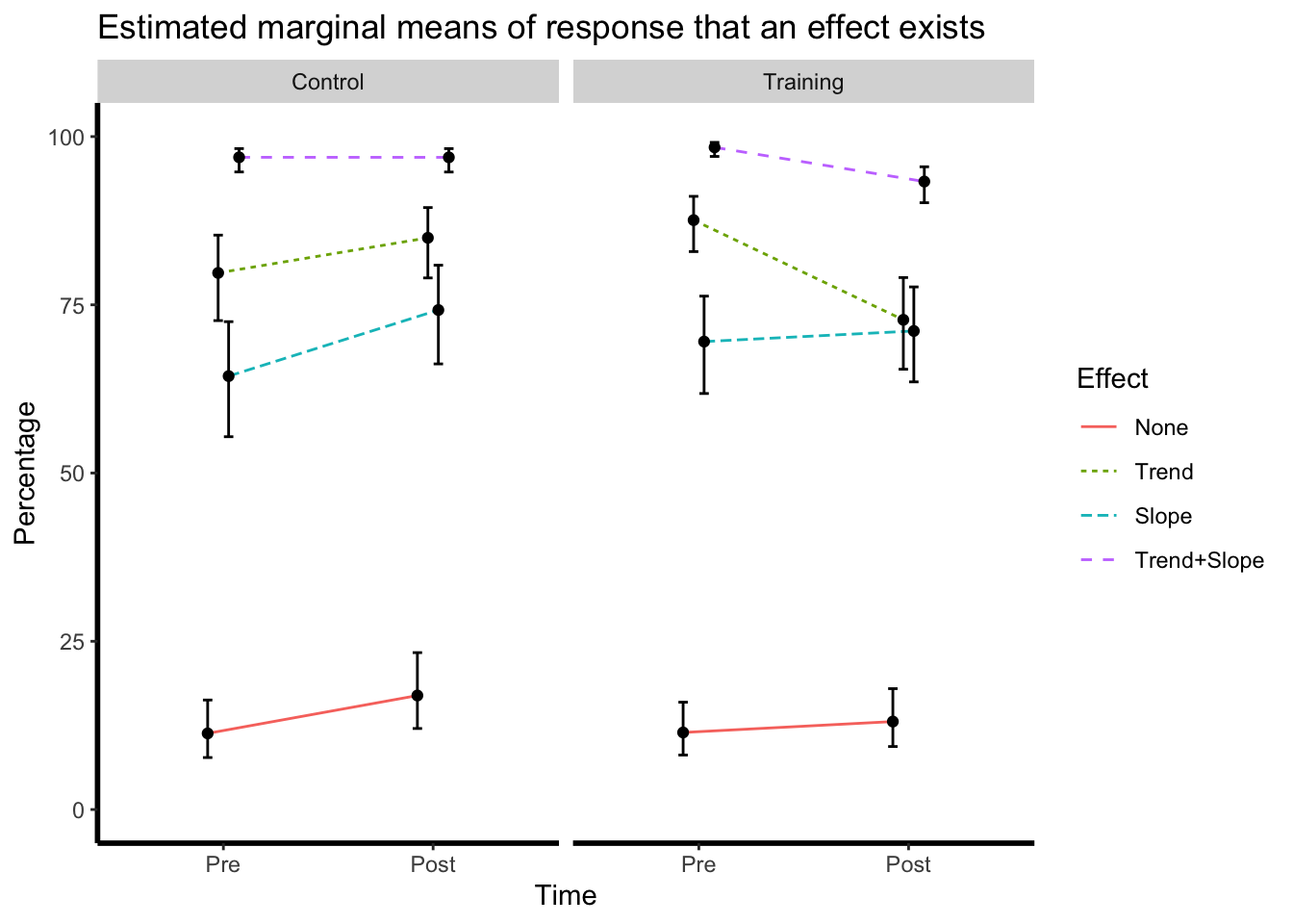
• Home
  • Projects
  • Publications
  • Software
  • Graduate Students
  • Private Blog

On this page

  • Deisgn
  • Descriptive analyses
  • “Traditional” Manova
  • Analyses with multilevel model
    • Estimated marginal means from the model

Analyze experimental data with a multilevel model

multilevel
R
experiments
statistics
Author

Jürgen Wilbert

Published

May 16, 2025

Abstract
Material for a brief explanation of how to analyse data from an experimental study with a multilevel model in R.
Load data
# Load the required library
library(tidyverse)
library(lmerTest)
library(sjPlot)
library(emmeans)
library(ez)

if (!("wmisc" %in% installed.packages())) devtools::install_github("jazznbass/wmisc")
if (!packageDate("wmisc") >= as.Date("2023-12-27")) devtools::install_github("jazznbass/wmisc")
library(wmisc)

dat_items <- readRDS(file.path("data-items.rds"))
dat_items <- dat_items %>%
  mutate(
    group = factor(
      group, levels = c(1, 0), 
      labels = c("Control", "Training")
    ),
    id_subject = sessionToken,
    time = factor(
      run, levels = c("pre", "post"),
      labels = c("Pre", "Post")
    ),
    item_effect = paste0(trend, slope),
    effect = factor(
      item_effect, 
      levels = c("00", "10", "01", "11"),
      labels = c("None", "Trend", "Slope", "Trend+Slope"))
  ) %>%
  arrange(id_subject,curr_timestamp)

dat_subjects <- dat_items %>% 
  filter(question == "effect") %>%
  group_by(id_subject, time, trend, slope, group) %>%
  summarise(
    prop = mean(response, na.rm = TRUE)
  ) %>% 
  mutate(id_subject = factor(id_subject), trend = factor(trend), slope = factor(slope)) %>%
  ungroup()


logit2prob <- function(logit){
  odds <- exp(logit)
  prob <- odds / (1 + odds)
  prob
}

Deisgn

Code
dat_items %>% filter(question == "effect") %>%
  group_by(sessionToken, group) %>%
  summarise(n = n()) %>%
  group_by(group) %>%
  summarise(n = n())
group n
Control 53
Training 64

DV 1: Yes/No ratings of single-case graphs “did the intervention have an effect?”

DV 2: 1-5 scale “How certain are you about your rating?”

Between IV 1: Intervention group with training in graphreading vs. controll group without training in graph reading.

Within IV 1: Pre-intervention vs. post-intervention

Within IV 2: Graph shows a trend-effect vs. no trend-effect

Within IV 3: Graph shows a slope-effect vs. no slope-effect

10 graphs per within condition: 2 x 2 x 2 x 10 = 80 Graphs

Descriptive analyses

Code
dat_items %>%
  filter(question == "effect") %>%
  group_by(group) %>%
  summarise(n = n()/ 80)
group n
Control 53
Training 64
Code
dat_items %>%
  filter(question == "effect") %>%
  group_by(group, effect, time) %>%
  summarise(
    mean_true = round(mean(response, na.rm = TRUE), 2)
  ) %>%
  ungroup() %>%
  pivot_wider(names_from = "time", values_from = "mean_true") %>%
    mutate(
    "Difference" = Post - Pre
    #sdt_category = rep(c("false alarm", "hit"), 4)
  ) %>%
  rename(Condition = group, Effect = effect) %>%
  relocate(Condition, Effect) %>%
  nice_table(
    file = "tab-desc-prop-response.docx", 
    title = "Proportion of graphs rated as showing an intervention effect"
  )
Table
Proportion of graphs rated as showing an intervention effect
Condition Effect Pre Post Difference
Control None 0.15 0.20 0.05
Control Trend 0.76 0.81 0.05
Control Slope 0.62 0.70 0.08
Control Trend+Slope 0.95 0.95 0.00
Training None 0.14 0.16 0.02
Training Trend 0.85 0.70 -0.15
Training Slope 0.66 0.68 0.02
Training Trend+Slope 0.98 0.91 -0.07

“Traditional” Manova

Code
dat_subjects %>% slice(1:20) %>% nice_table()
id_subject time trend slope group prop
03fRnek513UP Pre 0 0 Training 0.2
03fRnek513UP Pre 0 1 Training 0.8
03fRnek513UP Pre 1 0 Training 0.9
03fRnek513UP Pre 1 1 Training 1.0
03fRnek513UP Post 0 0 Training 0.4
03fRnek513UP Post 0 1 Training 0.7
03fRnek513UP Post 1 0 Training 0.5
03fRnek513UP Post 1 1 Training 0.9
0crR6ITOH4Hn Pre 0 0 Training 0.2
0crR6ITOH4Hn Pre 0 1 Training 0.9
0crR6ITOH4Hn Pre 1 0 Training 1.0
0crR6ITOH4Hn Pre 1 1 Training 1.0
0crR6ITOH4Hn Post 0 0 Training 0.6
0crR6ITOH4Hn Post 0 1 Training 0.9
0crR6ITOH4Hn Post 1 0 Training 1.0
0crR6ITOH4Hn Post 1 1 Training 1.0
15Eh1B5Nmc70 Pre 0 0 Training 0.0
15Eh1B5Nmc70 Pre 0 1 Training 0.8
15Eh1B5Nmc70 Pre 1 0 Training 1.0
15Eh1B5Nmc70 Pre 1 1 Training 1.0

Between subject factor is group and within subject factors are time, trend, and slope.

Code
fit <- ezANOVA(
  dat_subjects, 
  wid = id_subject, 
  dv = prop, 
  within = list(time, trend, slope), 
  between = group, 
  type = 3
)

nice_table(fit$ANOVA, decimals = 2)
Effect DFn DFd F p p<.05 ges
group 1.00 115.00 0.11 0.74 0.00
time 1.00 115.00 0.00 0.95 0.00
trend 1.00 115.00 1,124.79 0.00 * 0.58
slope 1.00 115.00 1,050.28 0.00 * 0.44
group:time 1.00 115.00 16.85 0.00 * 0.02
group:trend 1.00 115.00 0.01 0.91 0.00
group:slope 1.00 115.00 1.06 0.30 0.00
time:trend 1.00 115.00 26.39 0.00 * 0.01
time:slope 1.00 115.00 0.94 0.33 0.00
trend:slope 1.00 115.00 138.22 0.00 * 0.16
group:time:trend 1.00 115.00 5.27 0.02 * 0.00
group:time:slope 1.00 115.00 3.64 0.06 0.00
group:trend:slope 1.00 115.00 0.24 0.62 0.00
time:trend:slope 1.00 115.00 0.05 0.82 0.00
group:time:trend:slope 1.00 115.00 7.68 0.01 * 0.00

Analyses with multilevel model

Code
dat <- dat_items %>% 
  filter(question == "effect") %>%
  mutate(response = factor(response, labels = c("No", "Yes"))) %>%
  rename(Condition = group, Effect = effect, Time = time)

dat %>% slice(1:30) %>% select(id_subject, Condition, Time, Effect, response) %>% nice_table()
id_subject Condition Time Effect response
03fRnek513UP Training Pre Trend+Slope Yes
03fRnek513UP Training Pre Trend Yes
03fRnek513UP Training Pre Trend+Slope Yes
03fRnek513UP Training Pre Slope Yes
03fRnek513UP Training Pre Slope No
03fRnek513UP Training Pre Slope Yes
03fRnek513UP Training Pre None No
03fRnek513UP Training Pre Trend+Slope Yes
03fRnek513UP Training Pre Slope Yes
03fRnek513UP Training Pre None No
03fRnek513UP Training Pre Trend Yes
03fRnek513UP Training Pre Trend+Slope Yes
03fRnek513UP Training Pre Trend Yes
03fRnek513UP Training Pre Slope Yes
03fRnek513UP Training Pre None No
03fRnek513UP Training Pre Trend+Slope Yes
03fRnek513UP Training Pre None No
03fRnek513UP Training Pre Trend Yes
03fRnek513UP Training Pre Slope No
03fRnek513UP Training Pre Trend+Slope Yes
03fRnek513UP Training Pre None No
03fRnek513UP Training Pre Trend+Slope Yes
03fRnek513UP Training Pre None Yes
03fRnek513UP Training Pre Slope Yes
  1. Variables slope and trend are aggrgated into a new variable “effect” with for levels: “None”, “Trend”, “Slope”, “Trend+Slope”
Code
model <- glmer(
  response ~ Time * Condition * Effect + 
             (1|id_subject) + (1|id_subject:Time) + 
             (1|id_subject:Effect), 
  family = binomial,
  nAGQ = 0,
  data = dat, 
  na.action = na.omit
)

sjPlot::tab_model(
  model, 
  #file = "tab-reg-response.doc",
  show.se = FALSE, 
  show.ci = FALSE,
  show.stat = TRUE,
  show.df = FALSE,
  string.se = "se",
  string.est = "OR",
  string.stat = "t"
)

logistic models for assumed true responses (dummy contrasts)

  response
Predictors OR t p
(Intercept) 0.13 -9.58 <0.001
Time [Post] 1.60 2.26 0.024
Condition [Training] 1.01 0.05 0.963
Effect [Trend] 30.85 14.48 <0.001
Effect [Slope] 14.19 11.58 <0.001
Effect [Trend+Slope] 246.78 17.69 <0.001
Time [Post] × Condition
[Training]
0.73 -1.11 0.266
Time [Post] × Effect
[Trend]
0.90 -0.44 0.662
Time [Post] × Effect
[Slope]
1.00 -0.02 0.983
Time [Post] × Effect
[Trend+Slope]
0.62 -1.31 0.189
Condition [Training] ×
Effect [Trend]
1.77 1.75 0.080
Condition [Training] ×
Effect [Slope]
1.24 0.71 0.481
Condition [Training] ×
Effect [Trend+Slope]
1.93 1.42 0.155
(Time [Post] × Condition
[Training]) × Effect
[Trend]
0.36 -2.99 0.003
(Time [Post] × Condition
[Training]) × Effect
[Slope]
0.93 -0.22 0.825
(Time [Post] × Condition
[Training]) × Effect
[Trend+Slope]
0.31 -2.28 0.023
Random Effects
σ2 3.29
τ00 id_subject:Effect 0.59
τ00 id_subject:Time 0.29
τ00 id_subject 0.53
ICC 0.30
N id_subject 117
N Time 2
N Effect 4
Observations 9360
Marginal R2 / Conditional R2 0.444 / 0.611

Estimated marginal means from the model

Code
marginal_means <- emmeans(model, c("Time", "Effect", "Condition"),
  pbkrtest.limit = 9000,
  lmerTest.limit = 9000
)

means <- summary(marginal_means) |> as.data.frame()
means$probability <- logit2prob(means$emmean)
means$prob.ll <- logit2prob(means$asymp.LCL)
means$prob.ul <- logit2prob(means$asymp.UCL)

table_pre_post <- means %>%
  select(Condition, Effect, Time, probability) %>%
  pivot_wider(names_from = "Time", values_from = "probability") %>%
  mutate(Difference = round(Post-Pre, 2), Pre = round(Pre, 2), Post = round(Post, 2)) 

table_contrast <- marginal_means |> 
  pairs() |> 
  as.data.frame() |> 
    filter(contrast %in% c(
    "Pre None Control - Post None Control",
    "Pre None Training - Post None Training",
    "Pre Trend Control - Post Trend Control",
    "Pre Trend Training - Post Trend Training",
    "Pre Slope Control - Post Slope Control",
    "Pre Slope Training - Post Slope Training",
    "(Pre Trend+Slope Control) - (Post Trend+Slope Control)",
    "(Pre Trend+Slope Training) - (Post Trend+Slope Training)"
  )) %>% 
  mutate(
    across(where(is.numeric), ~round(.x, 2)),
    contrast = case_match(
      contrast,
      "Pre None Control - Post None Control" ~ "Control / none",
      "Pre None Training - Post None Training" ~ "Training / none",
      "Pre Trend Control - Post Trend Control" ~ "Control / trend",
      "Pre Trend Training - Post Trend Training" ~ "Training / trend",
      "Pre Slope Control - Post Slope Control" ~ "Control / slope",
      "Pre Slope Training - Post Slope Training" ~ "Training / slope",
      "(Pre Trend+Slope Control) - (Post Trend+Slope Control)" ~ "Control / trend+slope",
      "(Pre Trend+Slope Training) - (Post Trend+Slope Training)" ~ "Training trend+slope"
    )
  ) %>%
  rename("z ratio" = z.ratio, p = p.value) %>% 
  select(-1, -estimate, -df)

table_pre_post <- cbind(table_pre_post, table_contrast)
  nice_table(
    table_pre_post,
    file = "tab-marginal-means-response.docx",
    title = "Pre/post post-hoc contrasts of proportions of graphs rated as showing an intervention effect"
  )
Table
Pre/post post-hoc contrasts of proportions of graphs rated as showing an intervention effect
Condition Effect Pre Post Difference SE z ratio p
Control None 0.11 0.17 0.06 0.21 -2.26 0.65
Control Trend 0.80 0.85 0.05 0.20 -1.83 0.90
Control Slope 0.64 0.74 0.10 0.18 -2.58 0.41
Control Trend+Slope 0.97 0.97 0.00 0.33 0.01 1.00
Training None 0.11 0.13 0.02 0.20 -0.77 1.00
Training Trend 0.88 0.73 -0.15 0.18 5.48 0.00
Training Slope 0.70 0.71 0.02 0.16 -0.47 1.00
Training Trend+Slope 0.98 0.93 -0.05 0.33 4.49 0.00
Code
means %>% 
  mutate(Percentage = probability * 100) %>%
  ggplot(aes(x = Time, y = Percentage)) +
  geom_line(
    aes(color = Effect, group = Effect, linetype = Effect),
    position = position_dodge(0.2)
  ) + 
  geom_point(
    aes(group = Effect),
    position = position_dodge(0.2)
  ) + 
  geom_errorbar(
    aes(ymin = prob.ll * 100, ymax = prob.ul * 100), 
    width = 0.2,
    position = position_dodge2(0.2)
  ) +  
  facet_grid(cols = vars(Condition)) +
  ylim(c(0,100)) +
  theme(
    panel.background = element_rect(fill = "white"),
    legend.key  = element_rect(fill = "white"),
    axis.line.x = element_line(colour = "black", linewidth = 1),
    axis.line.y = element_line(colour = "black", linewidth = 1)
  ) + 
  xlab("Time") +
  ggtitle("Estimated marginal means of response that an effect exists")


© Jürgen Wilbert, last updated 2025-05-16