This feature is still in an experimental state. This means that the syntax structure, arguments, and defaults may change in future scan versions and may not be backward compatible.
Starting with version 0.63.0 scan included Bayesian regression analyses through the bplm() function (Bayesian Piecewise Linear Model).
In inferential statistics, a distinction is made between frequentist and Bayesian approaches. Frequentist statistics assess the probability of observing the data under the assumption that a null hypothesis (there is no effect or association) is true.
Bayesian statistics, on the other hand, begins with prior distributions that represent initial beliefs (priors) about the parameters of interest. These priors are then updated using observed data through Bayes’ theorem, which means that the initial beliefs about the parameters are adjusted in proportion to how well they explain the data, producing a posterior distribution that reflects both prior knowledge and new evidence. The Bayesian approach evaluates how well the data fit different parameter values by computing the likelihood of the data given these parameter estimates, rather than testing against a fixed null hypothesis.
The Bayesian approach is computationally intensive and often produces results that are practically similar to those of a frequentist analysis. However, it offers several advantages. In particular, when working with small samples, incorporating prior knowledge can improve parameter estimation. Additionally, Bayesian statistics does not require uniform distributional assumptions for all variables but allows each variable to have its own empirically derived distribution. Another advantage is its greater robustness against overspecified models, especially when too many predictors are included and exhibit high collinearity (intercorrelations) while the number of data points is limited.
These advantages make it worthwhile to use a Bayesian approach for single-case data.
The bplm() function computes a piecewise regression analysis. The syntax is quite similar to the plm() and hplm() functions. There you can find details about the general piecewise regression model, the interpretation of regression estimations, and the setting of contrast in models with more that two phases.
bplm() works for single-case dataframes with one case or multiple cases.
Note
bplm() uses the MCMCglmm package and function to compute the models. Parameters can be directly passed to that function with the arguments that are provided with bplm(). E.g., niter for setting the number of iterations or prior to set the priors.
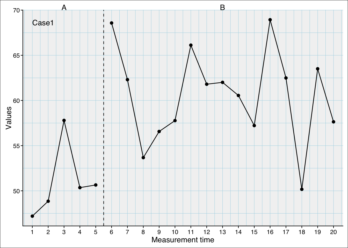
13.1 A one case analysis
Her is an example analyses of a one-case dataset:
bplm(exampleAB$Johanna)
Bayesian Piecewise Linear Regression

Contrast model: W (level: first, slope: first)
Deviance Information Criterion: 127.2107

B-structure - Fixed effects (values ~ 1 + mt + phaseB + interB)

                            B lower 95% CI upper 95% CI sample size     p
Intercept              54.419       46.405       61.675    1000.000 0.001
Trend (mt)              0.136       -3.099        3.417     710.368 0.904
Level phase B (phaseB)  7.603       -4.469       18.772    1000.000 0.200
Slope phase B (interB)  1.489       -1.897        4.756     696.272 0.366

R-Structure - Residuals

          SD lower 95% CI upper 95% CI
       5.368        3.437        7.122
In Bayesian terminology, the B-structure describes the fixed effects in a regression model and the R-structure the residuals of a model.
Let us take a closer look at the B-structure. As in any regression model, the coefficients represent the expected effects of the predictors on the outcome variable. In the present model, the intercept reflects the expected level of the outcome at time point zero in Phase A. The trend coefficient represents the expected change in the outcome for each additional measurement point within Phase A. The level coefficient (level effect) represents the change when Phase B begins. The slope coefficient (slope effect) represents the change in slope in Phase B compared to Phase A. Thus, the Phase B slope is given by the sum of the coefficients for trend and slope.
The CI values (here, CI stands for credible interval, not confidence interval) indicate how precisely the regression coefficients are estimated. The p value indicates how likely it is that the corresponding regression coefficient is on the opposite side of zero.
NoteMethodological details
We have to keep in mind that the Bayesian computational approach works somewhat differently from a linear mixed-effects regression estimated with maximum likelihood. The MCMC algorithm repeatedly generates new parameter values (i.e., iterations of parameter estimates) and evaluates how plausible these values are given the data and the prior assumptions. Over many iterations, this produces a sample from the posterior distribution of the model parameters. This posterior sample forms the basis for estimating the regression parameters and their uncertainty.
For this analysis, the maximum number of iterations was set to 13,000 (nitt = 13000). The first 3,000 iterations are discarded (burnin = 3000), because during this initial phase the Markov chain moves from its starting values toward the posterior distribution. From the remaining 10,000 iterations, only every tenth draw is stored (thin = 10) in order to reduce autocorrelation between consecutive samples.
The effective sample size (here the column sample size) indicates how many independent samples these draws correspond to after accounting for autocorrelation in the MCMC chain.
The B column shows the mean of a parameter from the posterior sample. The CI columns show the credible interval, which contains the central 95% of the posterior distribution after excluding the lowest 2.5% and the highest 2.5% of the sampled values.
The p column depicts two times the proportion of the posterior sample that are below zero (or for negative B values above zero). So the p-value is conceptually different from the probability statistics of a regression analysis that tests for the null-hypothesis. It is conceptually more similar to the p-value derived from a randomization test.
13.2 Multiple case analysis
For multilevel designs (i.e., multiple cases) a G-structure is reported which describes the between case effects (similar to the random effects of a linear mixed effect model but without the residual effects).
Here is an example of a multi-case dataset:
bplm(exampleAB_50)
Bayesian Piecewise Linear Regression

Contrast model: W (level: first, slope: first)
50 Cases

Deviance Information Criterion: 8574.866

B-structure - Fixed effects (values ~ 1 + mt + phaseB + interB)

                            B lower 95% CI upper 95% CI sample size     p
Intercept              48.374       45.386       51.455        1000 0.001
Trend (mt)              0.583        0.354        0.798        1000 0.001
Level phase B (phaseB) 14.024       12.851       15.346        1000 0.001
Slope phase B (interB)  0.897        0.679        1.137        1000 0.001

G-Structure - Random effects (~case)

 Parameter     SD lower 95% CI upper 95% CI
 Intercept 10.318         8.28       12.369

R-Structure - Residuals

          SD lower 95% CI upper 95% CI
       5.301        5.113        5.501
13.3 Setting priors
The following example show the influence of priors on paramameter estimation. Firstly, we create a random case from previously defined parameters:
The starting value (intercept) is 50 (the standard deviation is 10). The level effect for Phase B is one standard deviation (that is, 10 points) and there is neither a slope nor a trend effect. Random noise is introduced with 20% measurment error (reliability is 0.8).
set.seed(123) #set random seed for replicability of the exampledes <-design(start_value =50, s =10,level =list(A =0, B =1), trend =list(0),slope =list(0),rtt =0.8)scdf <-random_scdf(des)scplot(scdf)
Here are the estimations from a Bayesian model without informative priors:
bplm(scdf)
Bayesian Piecewise Linear Regression

Contrast model: W (level: first, slope: first)
Deviance Information Criterion: 128.5297

B-structure - Fixed effects (values ~ 1 + mt + phaseB + interB)

                            B lower 95% CI upper 95% CI sample size     p
Intercept              49.323       40.969       57.548     905.804 0.001
Trend (mt)              0.826       -2.195        4.368    1146.096 0.618
Level phase B (phaseB)  8.238       -4.645       19.994    1684.465 0.186
Slope phase B (interB) -0.984       -4.650        2.130    1109.566 0.532

R-Structure - Residuals

          SD lower 95% CI upper 95% CI
       5.599        3.457        7.517
Now we introduce our prior knowledge: an intercept of 50, a trend and slope effect of 0, and a level effect of 10. We also assume that our prior is quite uncertain (i.e., a weakly informative prior). mu sets the prior values for the four parameters in the order they appear in the regression model. V is a diagonal matrix of the variances of these estimates. The V matrix sets the strength of the prior. Here we set values of 100, which is one standard deviation (\(SD^2 = 10^2 = 100\)).
As we are setting the fixed parameters (B-structure) of the model, we enclose these settings in a list with the name B. The argument prior takes a list of lists, so we need to enclose the B-structure in a list as well.