5  Creating a single-case data plot

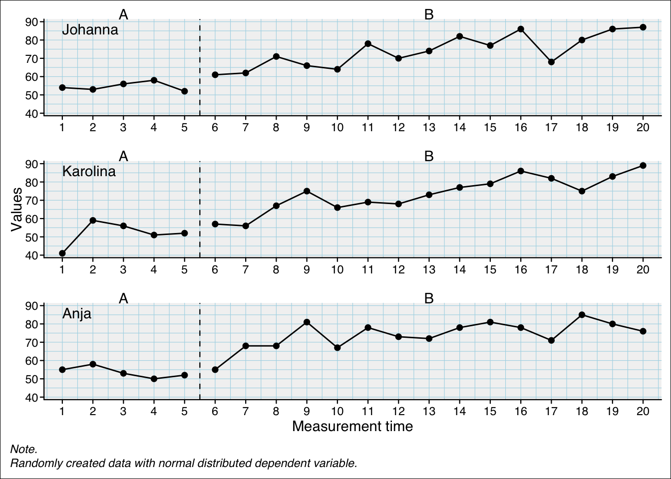
Plotting the data is a first important approach to single-case analysis. The scplot package has a set of functions to visualizes single-case data. It takes your sccdf an draws a time series plot and, if the scdf contains more than one case, a multiple baseline plot is created.

scplot is an add-on package to scan for visualizing single-case data.¹

5.1 Install scplot

splot is available from the CRAN repository. Execute install.packages("scplot") to install it.

If you are more adventures, you can install the developmental version of scplot from github.The project is hosted at https://github.com/jazznbass/scplot. You can install it with pak::pak("jazznbass/scplot") from your R console. Make sure you have the package pak installed before². The scplot package has to be compiled. When you are running R on a Windows machine you also have to install Rtools. Rtools is not an R package and can be downloaded from CRAN at https://cran.r-project.org/bin/windows/Rtools/.

The following chapter has been written with scplot version 0.7.0. If you have problems replicating the examples, please update to this version.

5.2 Basic principal

TipThe scplot function call:

scplot(object, …)

You start by providing an scdf object (see Section 3.2) to the scplot() function (e.g. scplot(exampleAB)). This already creates a default plot.

scplot(exampleAB)

Now you use a series of pipe-operators (|>) to apply functions that add elements and change characteristics of the resulting plot. For example:

scplot(exampleABC) |>
  add_title("My plot") |>
  set_xlabel("Days", color = "red", size = 1.3)

Here is an overview of possible functions:

Table 5.1: scplot functions

Function	What it does ...
set_dataline	Change the default dataline/ add an additional dataline
add_statline	Add a line or curve representing statistical parameters
add_arrow	Add an arrow to a specific case at a specific position
add_line	Add a line to a specific case
add_grid	Add a grid to the plot pannel
add_labels	Add value labels to each data-point
add_legend	Add a plot legend
add_marks	Mark specific data points of specific cases
add_ridge	Colour the area below the dataline
add_text	Add text to a specific case at a specific position
add_title	Add a title above the plot
add_caption	Add a caption below the plot
set_xlabel/ set_ylabel	Change and style axis labels
set_xaxis/ set_yaxis	Set the value range, increments etc. of the x- and y-axis
set_background	Set colour and texture of the plot background
set_panel	Set colour and texture of the plot panel
set_phasenames	Rename and style the phases
set_casenames	Rename and style the phases
set_separator	Style the vertical separator line between phases
set_theme	Apply a predefined visual theme
set_theme_element	Style specific elements of the plot
as_ggplot	Return a ggplot2 object for further processing
new_theme	Create/define a new visual theme

5.3 Visual characteristics

All text, line, dot, and area elements have a set of arguments to change visual characteristics.

Text arguments can be applied to the following functions: add_caption(), add_labels(), add_legend(), add_text(), add_title(), set_xlabel(), set_ylabel(), set_phasenames(), set_casenames().

Possible arguments are:

Table 5.2: Arguments for text elements

Argument	What it does ...
color	Change color. Either a color name or a color code (e.g. 'red' or '#110044').
size	Relativ size to the base text size.
family	The font ('serif', 'sans', 'mono')
face	The font face ('plain', 'bold', 'italic', 'bold.italic')
hjust	Horizontal alignment (0 = left, 0.5 = centered, 1 = right)
vjust	Vertical alignment (0 = upper, 0.5 = centered, 1 = lower)

Line arguments can be applied to the following functions: set_dataline(), add_statline(), add_line(), add_arrow(), add_ridge(), set_xaxis(), set_yaxis(), set_separator().

Table 5.3: Arguments for line elements

Argument	What it does ...
color	Either a color name or a color code (e.g. 'red' or '#110044').
linewidth	Relativ width of the line.
linetype	Linetype ('solid', 'dashed', 'dotted')

Point arguments can be applied to the following functions: set_dataline(), add_statline(), add_marks(), add_arrow().

Table 5.4: Arguments for point elements

Argument	What it does....
color	Either a color name or a color code (e.g. 'red' or '#110044').
linewidth	Relativ width of the line.
linetype	Linetype ('solid', 'dashed', 'dotted')

Figure 5.1: Some possible shapes

5.4 Set and add datalines

TipThe set_dataline function call:

set_dataline(
  object,
  variable = NULL,
  line,
  point,
  type = “continuous”,
  label = NULL,
  show_gaps = FALSE,
  …
)

By default, the single-case plot will depict the main dependent variable as defined in the scdf object. For changing this default behaviour or adding a second data line, use the set_dataline() function. The function takes the argument variable (with the main dependent variable as a default) which must correspond to a variable name within the applied scdf.

scplot(exampleAB_add) |>
  set_dataline("depression")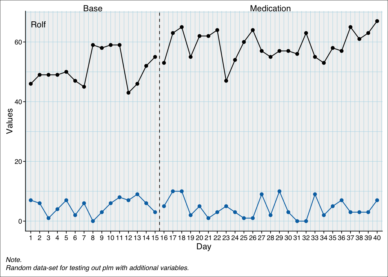

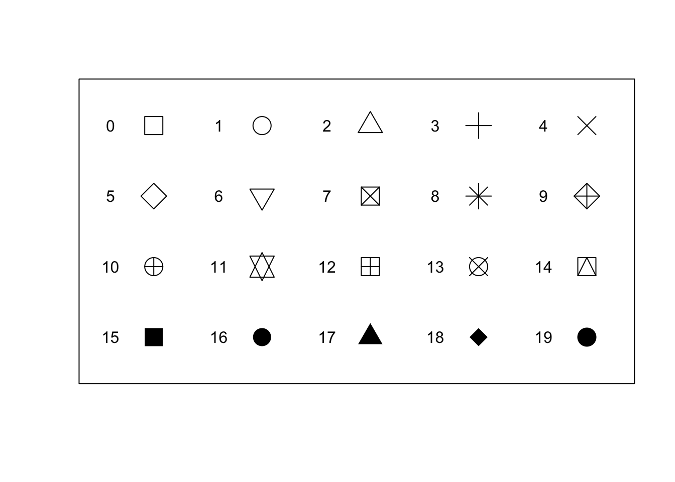
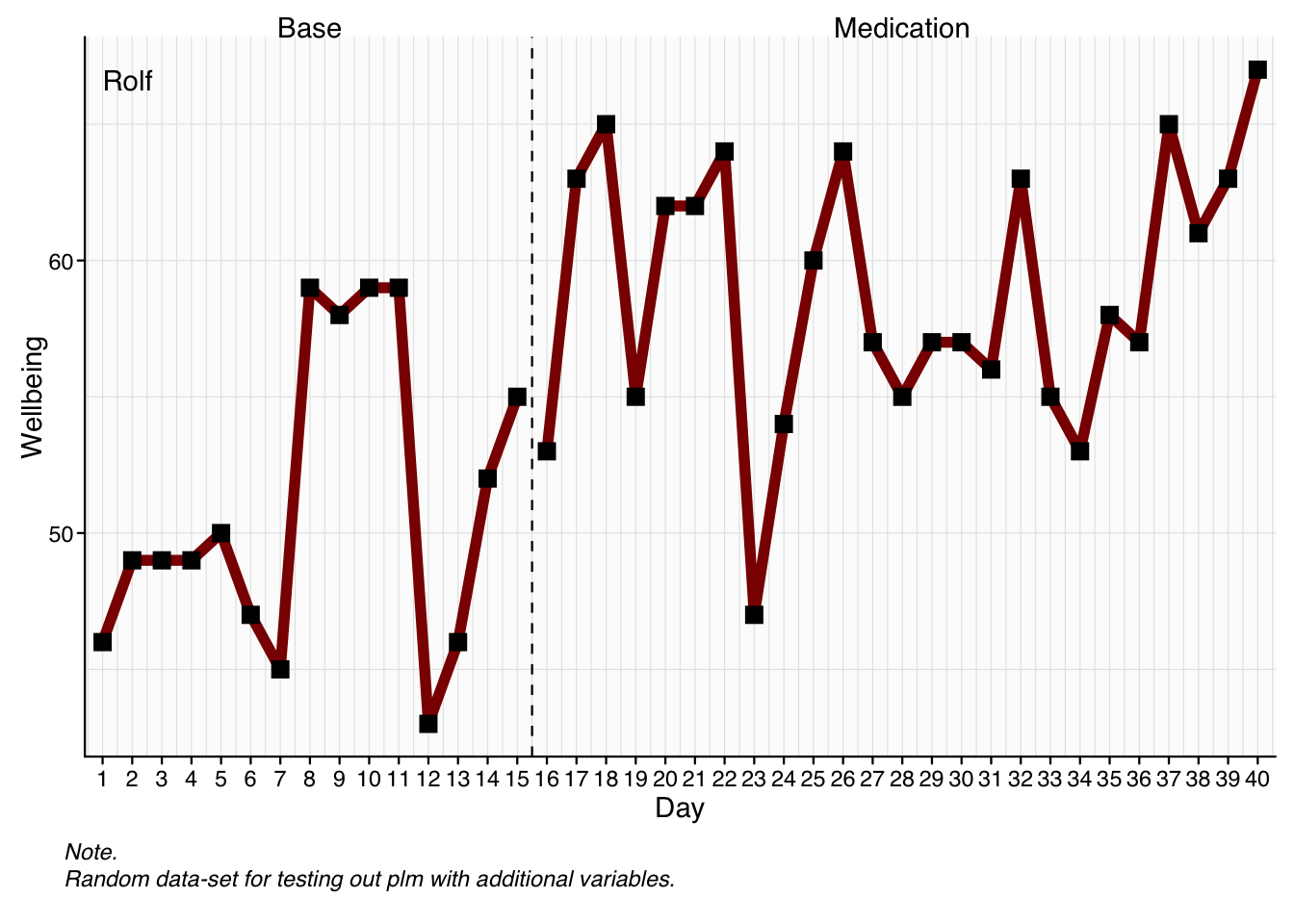
Styling parameters like line and point colour will be set automatically based on the applied graphic theme. We will learn later about how to change and modify these themes. If you want to directly change the styling parameters, you can use the line and point arguments which take lists with styling parameters. For line, the parameters are colour, linewidth, linetype, lineend, and arrow. For point the parameters are colour, size, and shape.

scplot(exampleAB_add) |>
  set_dataline(
    line = list(colour = "darkred", linewidth = 2), 
    point = list(colour = "black", size = 3, shape = 15)
  )

5.5 Add statlines

TipThe add_statline function call:

add_statline(
  object,
  stat = c(“mean”, “median”, “min”, “max”, “quantile”, “sd”, “mad”, “trend”, “moving mean”, “moving median”, “loreg”, “lowess”, “loess”, “trendA”, “trendA theil-sen”, “trendA bisplit”, “trendA trisplit”),
  phase = NULL,
  color = NULL,
  linewidth = NULL,
  linetype = NULL,
  variable = NULL,
  label = NULL,
  segmented = NULL,
  case = NULL,
  …
)

Adding statlines is an important way to visualize statistical parameters of the data. The add_statline() function takes the argument stat which specifies the statistic to be visualized. The following sections show some examples for different statistics.

5.5.1 A line for each phase

A first approach is to draw a line for each phase. This can be achieved with the following statistics mean, min, max, median, sd, quantile, and trend.

scplot(exampleABC) |>
  add_statline("mean") |>
  add_statline("max") |>
  add_statline("min") |> 
  add_statline("median")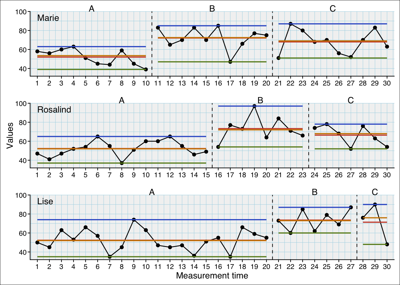

5.5.2 A line for a specific phase

If you specify a specific phase, the statistic will be calculated for this phase only and the line will be drawn across the whole plot. This is usually used to draw a baseline as a reference for all other phases but can also be used with any phase (e.g., to draw a line with the mean of the intervention phase across the whole plot or the median of multiple combined intervention phases).

If you want to draw a line based on all phases (i.e., all values), set phase = "all".

The following example sets a line with the mean of phase A, the maximum of phases B and C, the minimum of phases 2 and 3, and the median of all phases:

scplot(exampleABC) |>
  add_statline("mean", phase = "A") |>
  add_statline("max", phase = c("B", "C")) |>
  add_statline("min", phase = c(2, 3)) |> 
  add_statline("median", phase = "all") |>
  add_legend()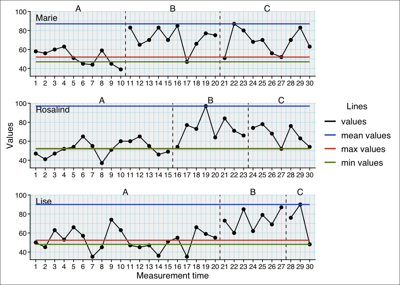

5.5.3 Trend-lines

By default, the trend statistic will give you a linear regression line (ordinary least squared method) for each phase. You can specify other methods for calculating the trend line with the method argument. Possible values are theil-sen, bisplit, and trisplit. The theil-sen method calculates a median based regression line. The bisplit and trisplit methods split the data into two or three parts and calculates a regression line for the median values of the first and last part. These methods are more robust against outliers but can also be less precise than the ordinary least squared method.

scplot(exampleABC) |> 
  add_statline("trend") |> 
  add_statline("trend", method = "theil-sen") |> 
  add_statline("trend", method = "bisplit") |> 
  add_statline("trend", method = "trisplit")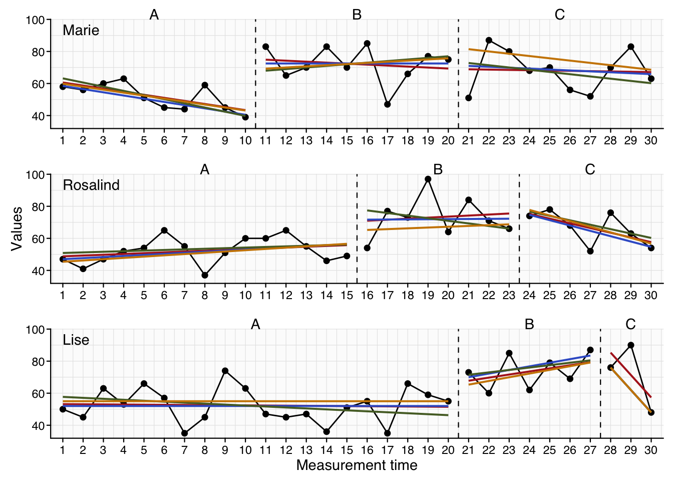 

If you want to draw a trend line for a specific phase, set the phase argument to the respective phase. The following example draws a linear regression line for each phase and an additional linear regression line for the baseline trend phase A with the OLS and Theil-Sen methods:

scplot(exampleABC) |>
  add_statline("trend") |>
  add_statline("trend", phase = "A", method = "theil-sen") |>
  add_statline("trend", phase = "A")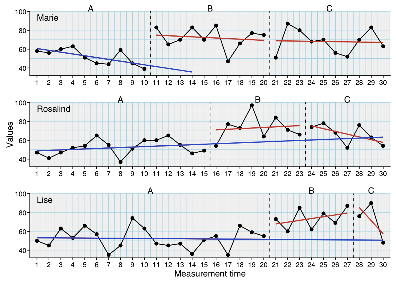

5.5.4 Smoothed curves

Smoothed curves try to capture the general pattern of the data by fitting a curve to the data points. scplot provides several methods for calculating smoothed curves. Possible values for the stat argument are moving mean, moving median, loess, lowess.

Moving averages (based on the mean or median) compute a value for each data point using the surrounding observations. The lag argument specifies how many neighboring points are included on each side of the focal point. For example, lag = 2 means that the average is calculated from the focal data point, the two preceding values, and the two following values.

loess and lowess fit a local regression to the data. The arguments span (for loess) and f (for lowess) specify the proportion of neighbouring observations used to fit each local regression.

scplot(exampleABC) |>
  add_statline("loess") |>
  add_statline("moving mean")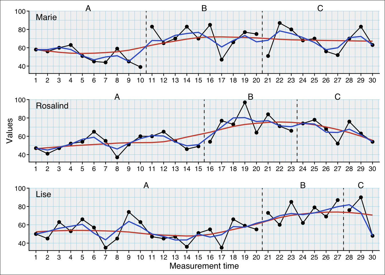

5.5.5 Refine with additional arguments

Some of the statistics allow additional arguments to specify parameters:

Statistic	Argument	What it does …
mean	trim	Trims the mean. trim = 0.10 calculates a 10% trimmed mean.
quantile	probs	Probability. probs = 0.25 calculates the 25% quantile.
moving mean, moving median	lag	Lag surrounding the estimated value. lag = 2 will calculate mean or median based on the two values before and after the to be replaced value.
loess	span	Proportion of the surrounding point to estimate a value.
lowess	f	Proportion of the surrounding point to estimate a value.

scplot(exampleABC) |>
  add_statline("moving mean", lag = 1) |>
  add_statline("quantile", probs = 0.75)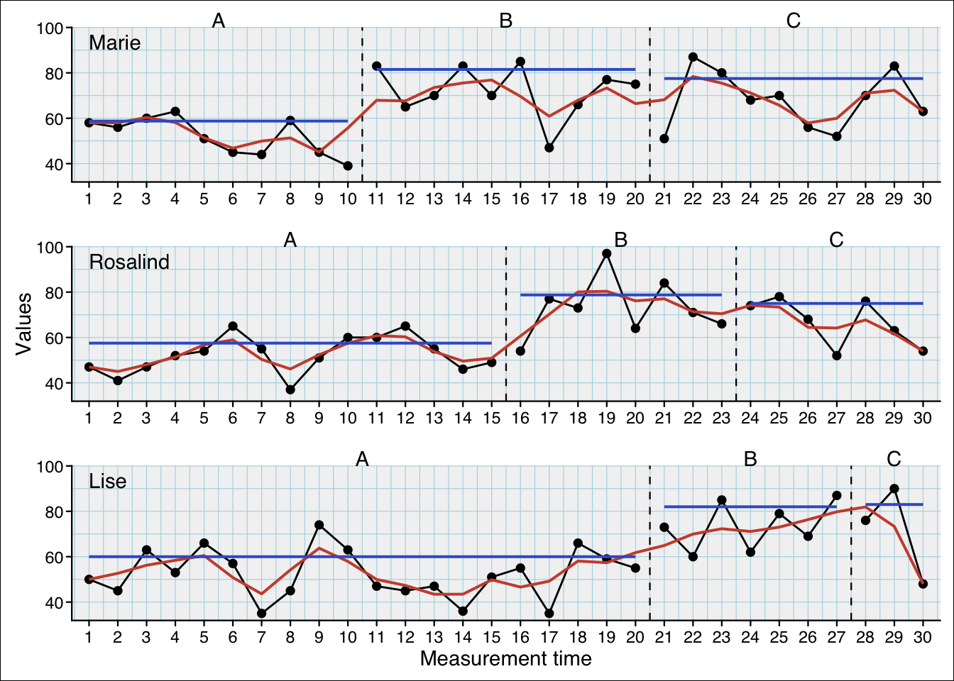

5.5.6 Specify data-line

If you do not specify the variable argument, the statline refers to the default first data-line.

scplot(exampleAB_add) |>
  set_dataline("cigarrets") |>
  add_statline("mean", variable = "cigarrets") |>
  add_statline("trend")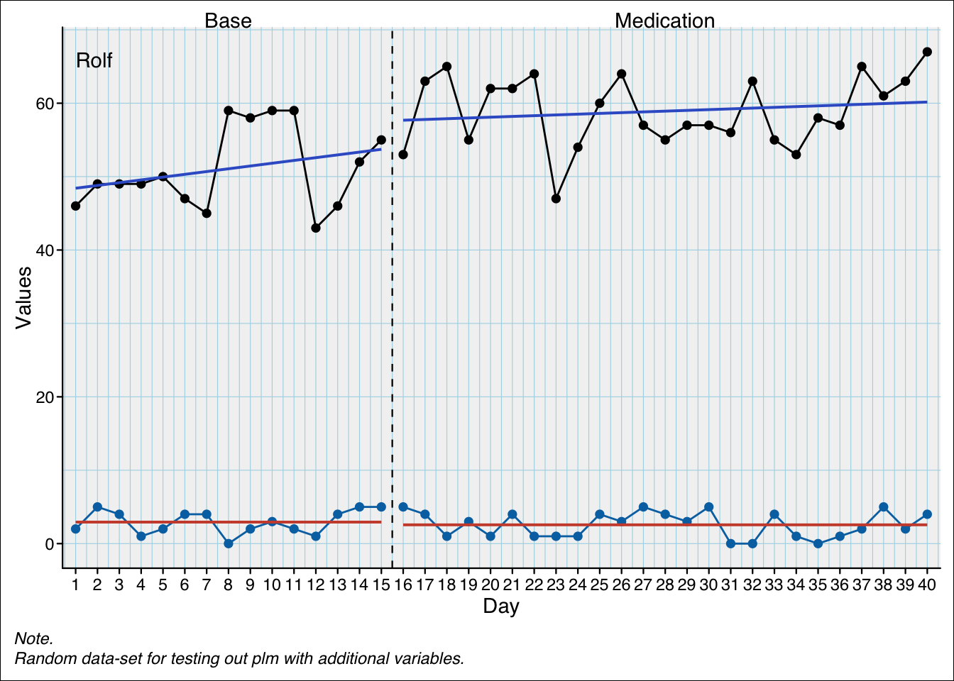

5.5.7 Choose cases

By default, the statline is drawn for all cases. You can specify a specific case with the case argument. This is particularly useful for multiple baseline plots.

scplot(exampleAB) |>
  add_statline("mean", case = 1) |>
  add_statline("trend", case = 2) |>
  add_statline("max", phase = "A", case = 3) |> 
  add_legend()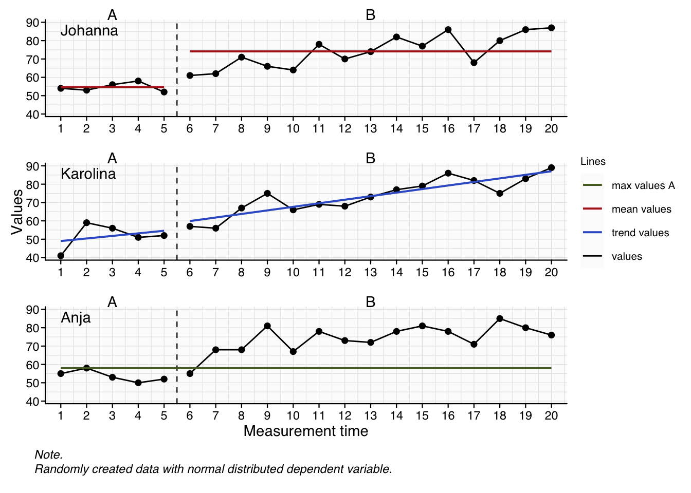

5.5.8 Segmented lines

The lines can be drawn with gaps between the phases by setting segmented = TRUE. This can be applied to all statlines but is particularly useful for statistics that visualize the changes between phases. The defaults for trend depend on the stat and phase settings.

scplot(exampleABC) |>
  add_statline("loess", segmented = TRUE, case = 1) |>
  add_statline("trend", segmented = FALSE, case = 2) |>
  add_statline("trend", phase = "B", segmented = TRUE, case = 3)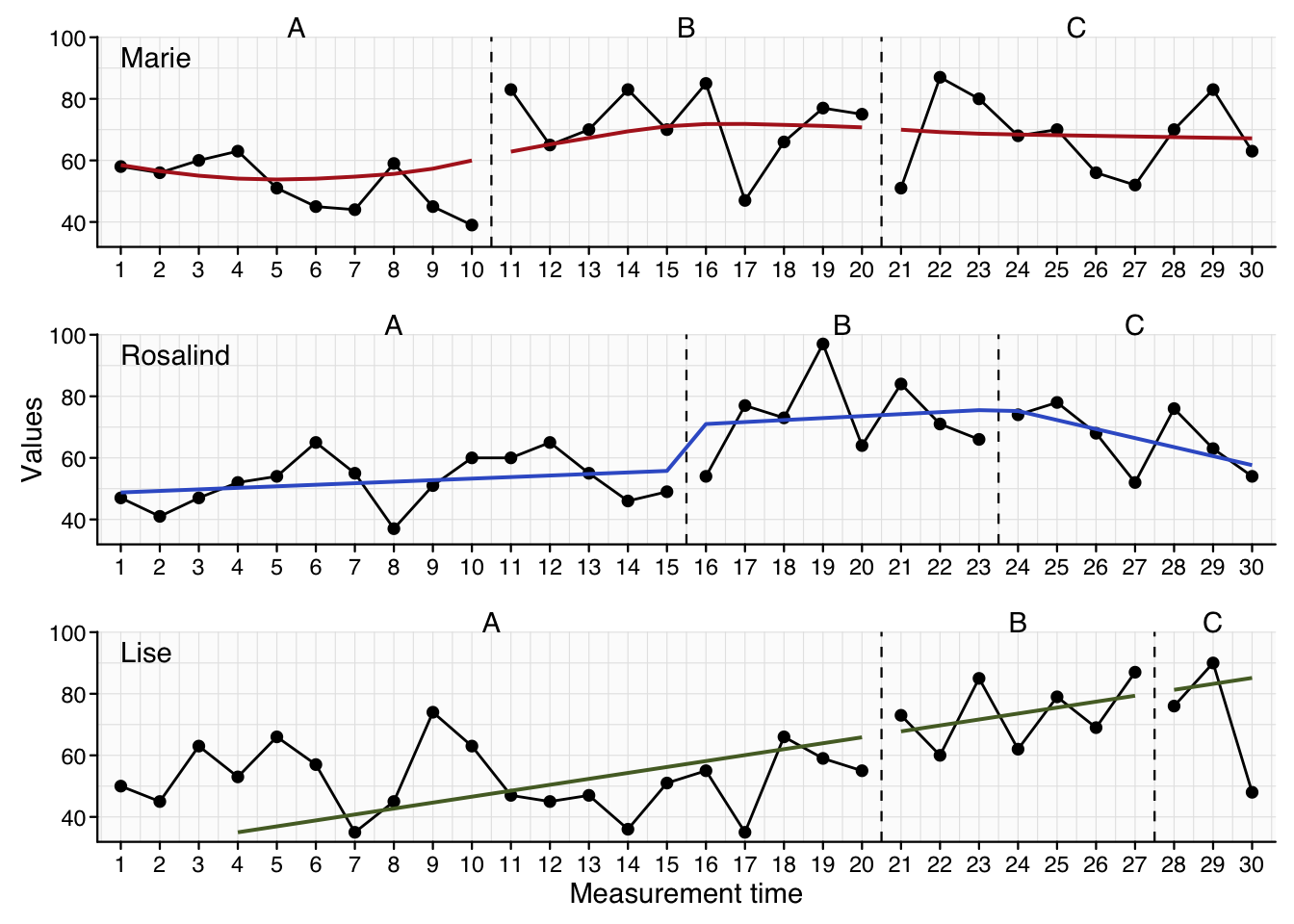

5.6 Annotate and mark

5.6.1 Add marks

The positions argument can take a numeric vector:

scplot(exampleABC) |>
  add_marks(case = 1, positions = c(7, 12)) |>
  add_marks(case = 3, positions = c(3, 17), color = "blue", size = 7)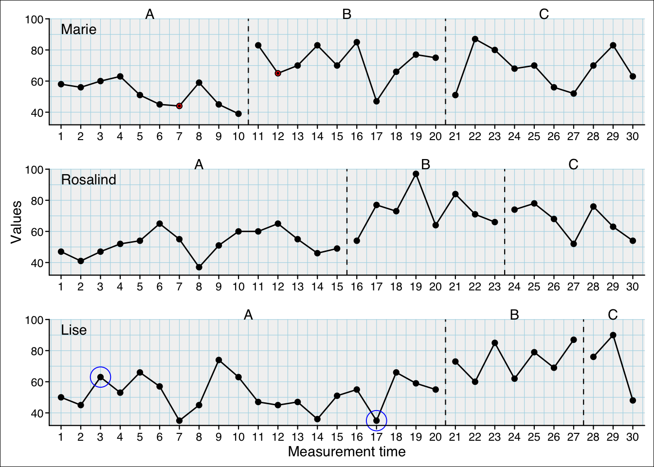

The positions argument can also be a string containing a logical expression. This will be evaluated and the respective positions will be marked.

scplot(exampleABC) |>
  add_marks(case = 1, positions = "mt > 15") |>
  add_marks(case = 2, positions = 'phase == "B"', color = "green", size = 5) |>
  add_marks(case = 3, positions = "values > quantile(values, probs = 0.80)", color = "blue", size = 7) |>
  add_marks(case = "all", positions = "values < quantile(values, probs = 0.20)", color = "yellow", size = 7) |>
  add_caption("red: mt > 15 in case 1; 
green: phase 'B' in case 2; 
blue: values > 80% quantile of case 3; 
yellow: values < 20% quantile of all cases")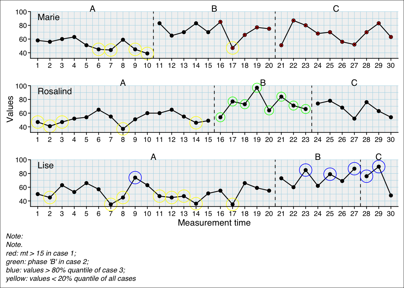

And the positions argument can take the results from a scan outlier analyses and mark the positions of the outliers of each case:

scplot(exampleABC_outlier) |> 
  add_marks(positions = outlier(exampleABC_outlier), size = 3)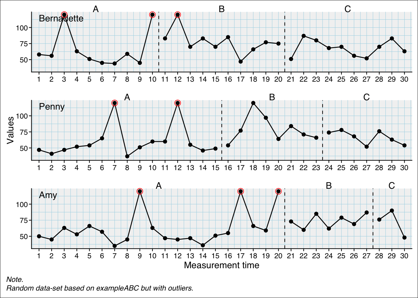

5.6.2 Add text

scplot(exampleABC) |>
  add_text("Here!", case = 2, x = 10, y = 80, color = "red")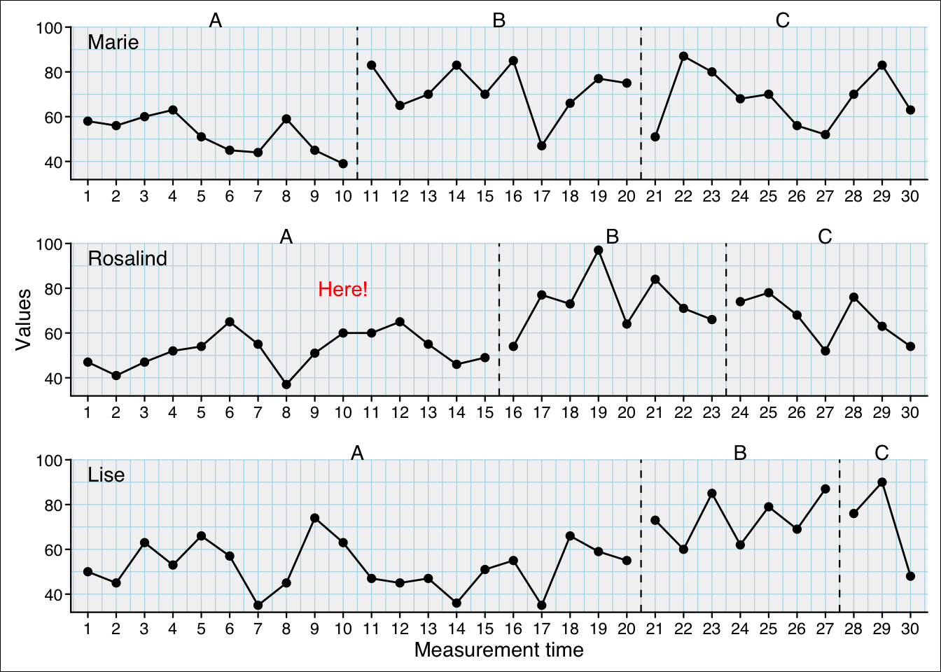

5.6.3 Add line

Draw lines either by providing starting (x0 and y0) an end coordinates (x1 and y1) or a horizontal (hline) or vertical (vline) position:

scplot(exampleABC) |>
  add_line(case = 1, x0 = 6, y0 = 90, x1 = 3, y1 = 63, color = "red") |> 
  add_line(case = 2, hline = 80, color = "blue") |> 
  add_line(case = 3, vline = 15, color = "darkgreen")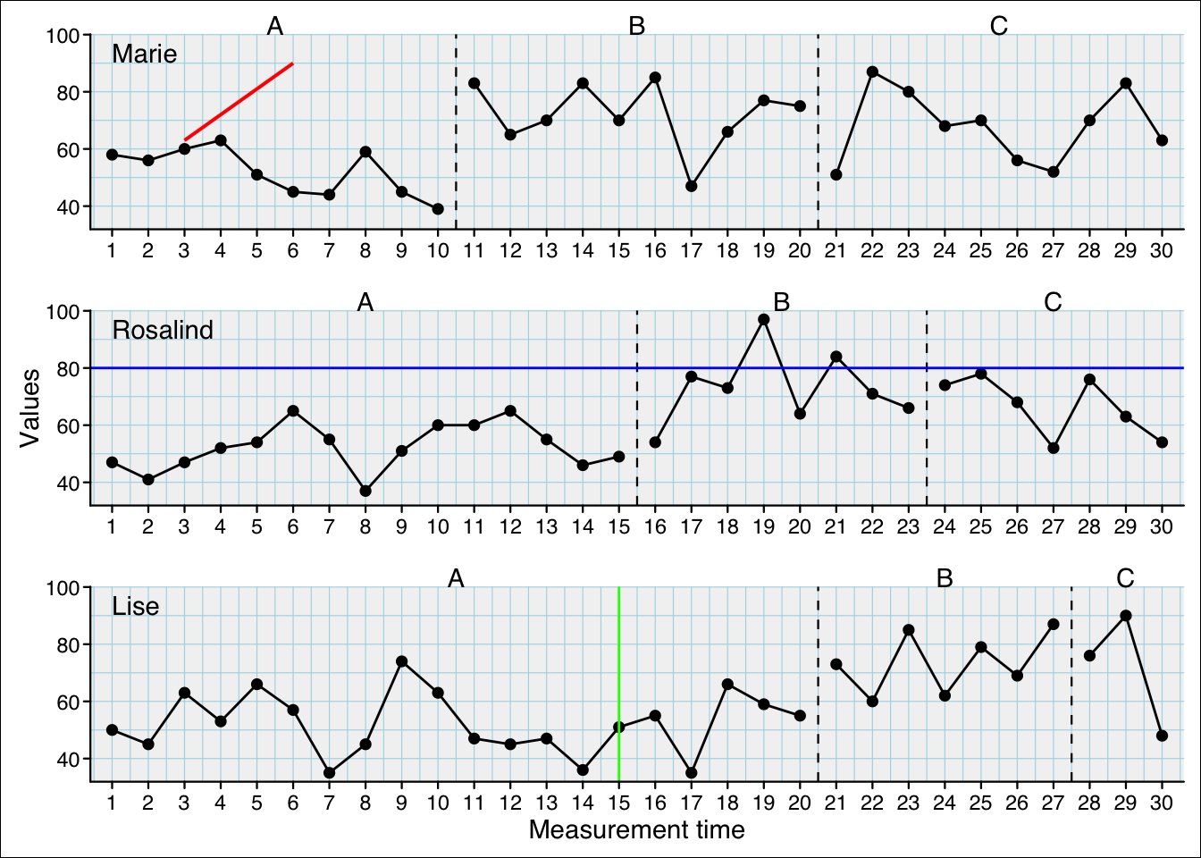

Draw an arrow:

scplot(exampleABC) |>
  add_arrow(case = 1, x0 = 6, y0 = 90, x1 = 3, y1 = 63) |>
  add_text("Problem", case = 1, x = 6, y = 94, color = "red", size = 1, hjust = 0 ) 

5.7 Change appearance of basic plot elements

5.7.1 Data line

scplot(exampleABC) |>
  set_dataline(color = "blue", linewidth = 1, linetype = "dotted", 
               point = list(colour = "red", size = 1, shape = 2) )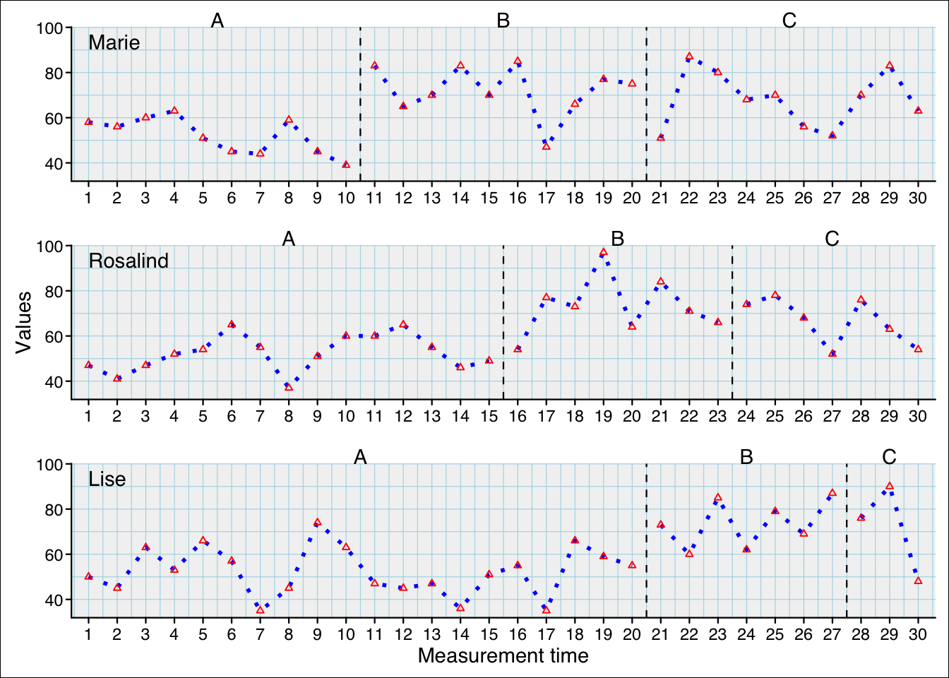

# Equivalent_
# scplot(exampleABC) |>
#   set_dataline(line = list(colour = "blue", linewidth = 1, linetype = "dotted"), 
#                point = list(colour = "red", size = 1, shape = 2)) 

5.7.2 Background

The background ist the complete area of the plot including a frame.

scplot(exampleABC) |>
  set_background(fill = "grey90", color = "black", linewidth = 2)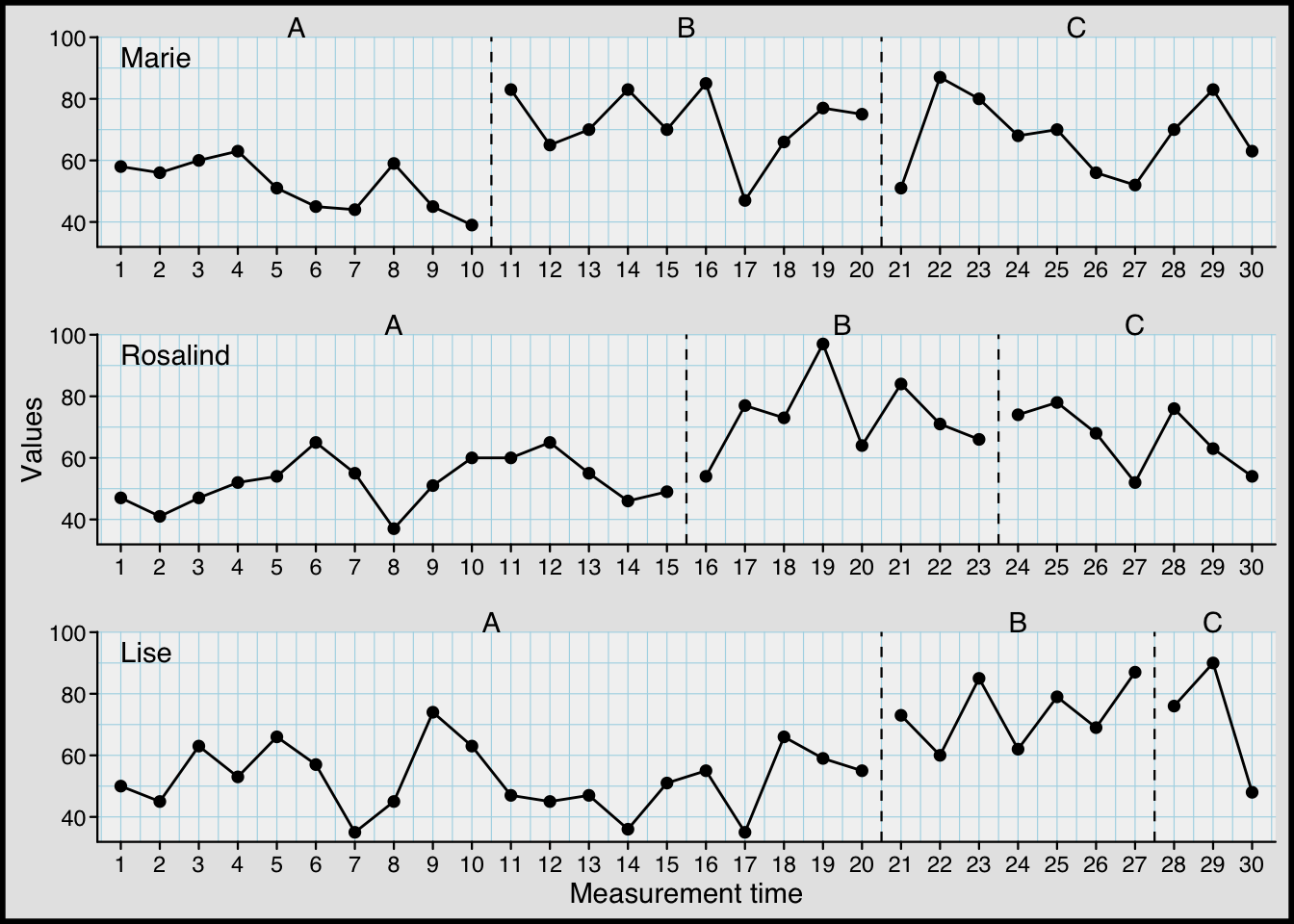

5.7.3 Panel

The panel refers to the coordinate system.

scplot(exampleABC) |>
  set_panel(fill = "tan1", colour = "palevioletred", linewidth = 2)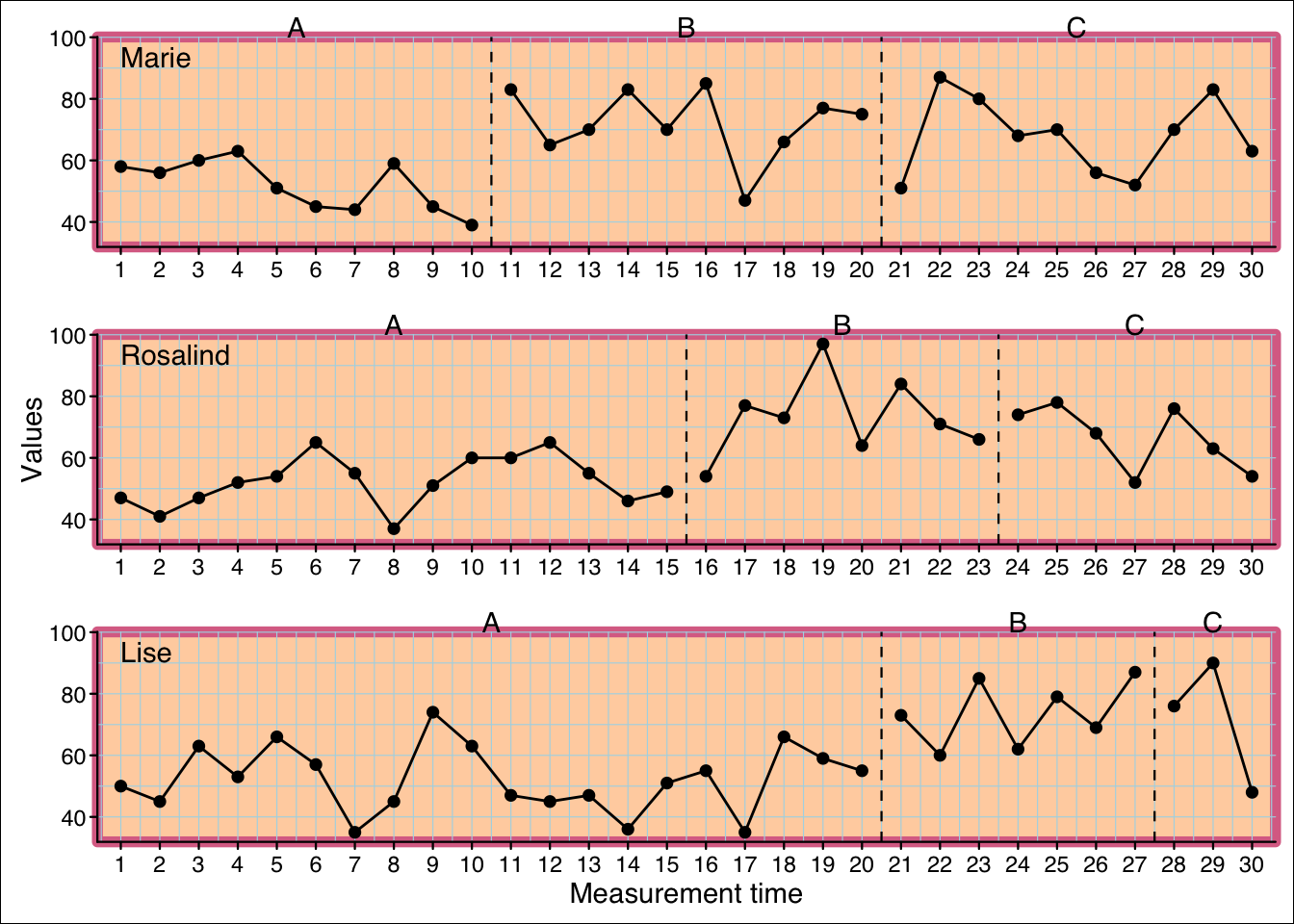

You can specify a different panel color for each phase by providing a vector to the fill argument:

scplot(exampleABC) |>
  set_panel(fill = c("grey80", "white", "blue4"))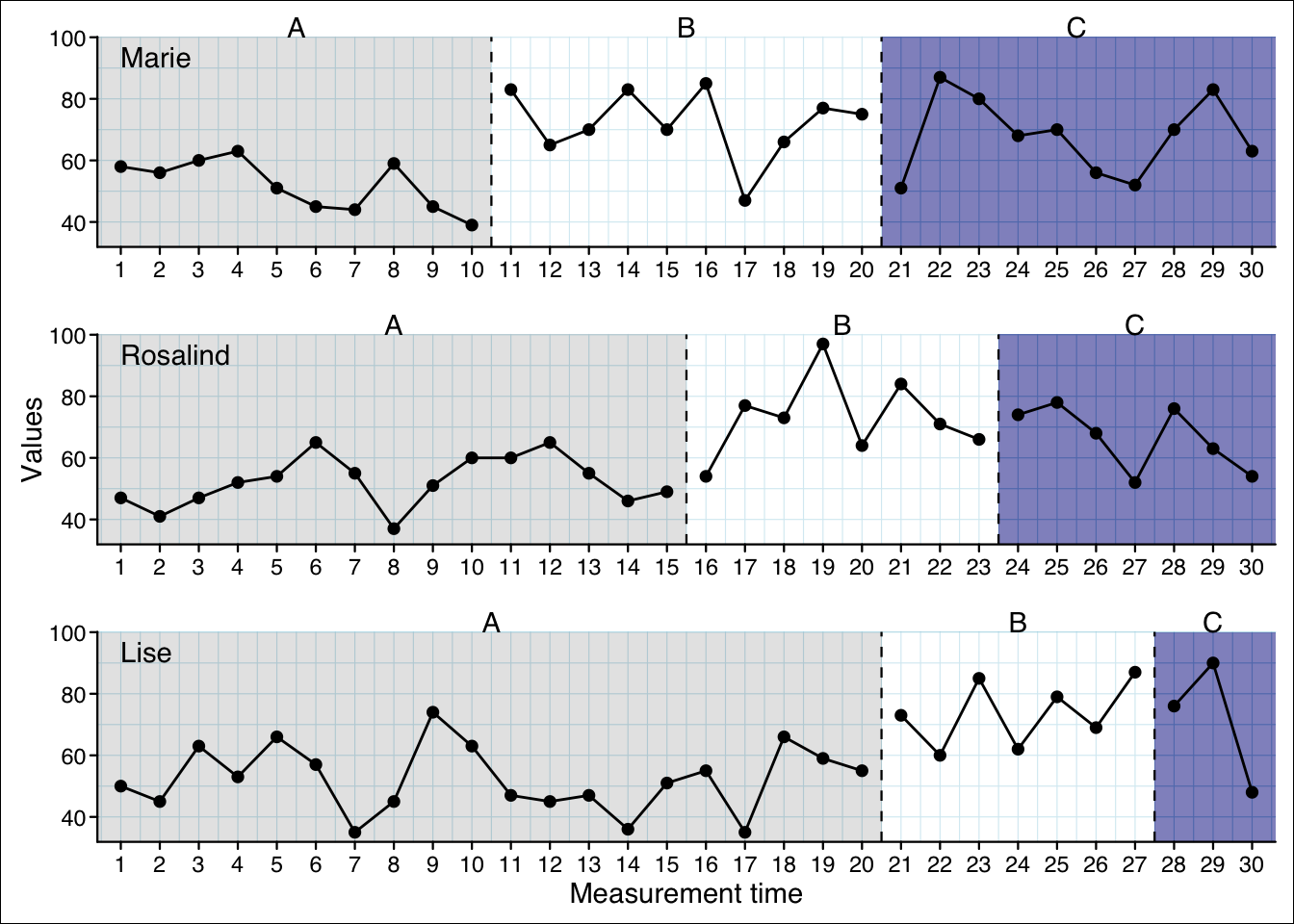

Note: The colours are 50% transparent. So they might appear different.

5.8 Themes

Themes are complete styles that define various elements of a plot.

Function set_theme("theme_name")

Possible themes:

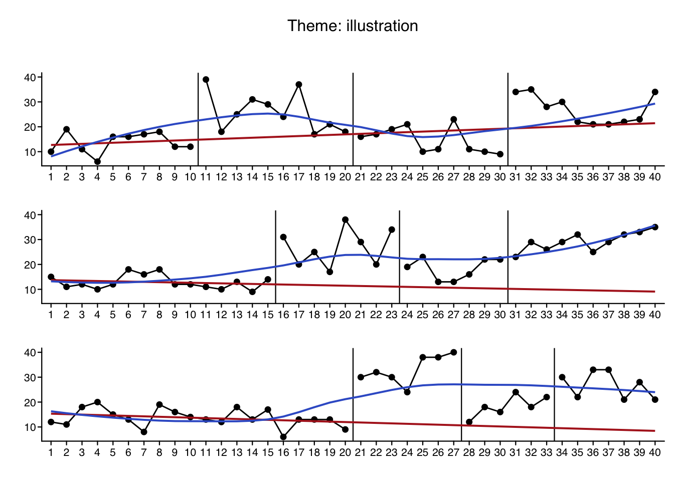
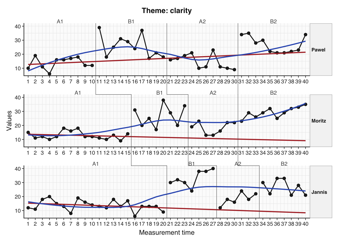
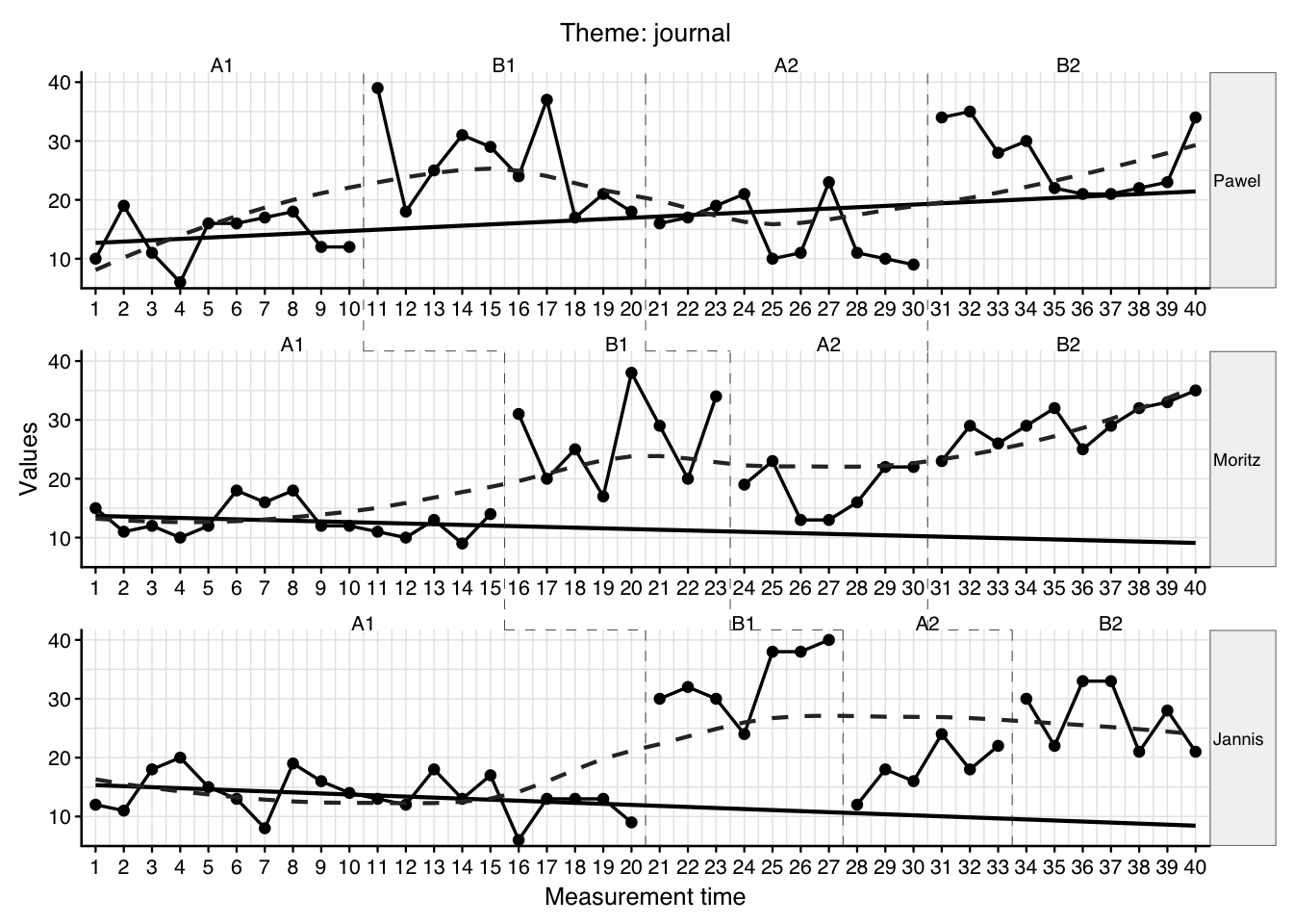
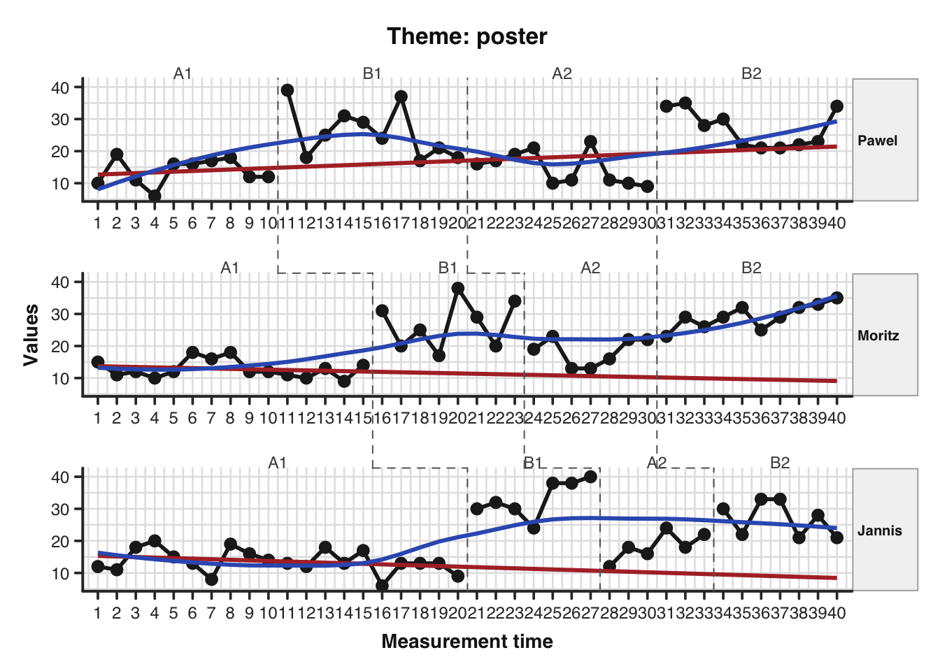
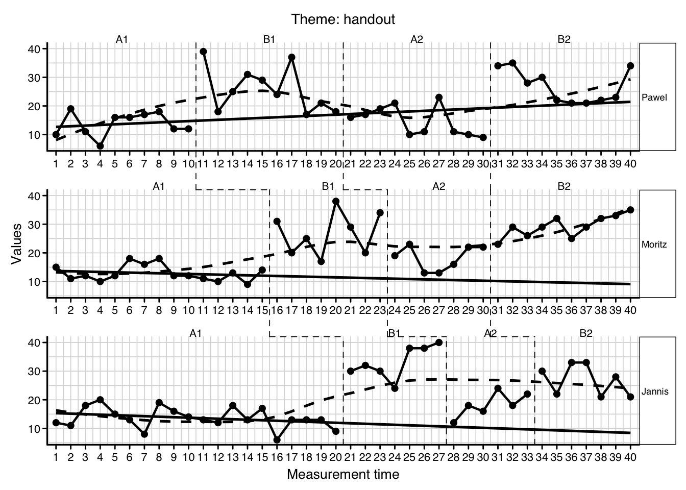
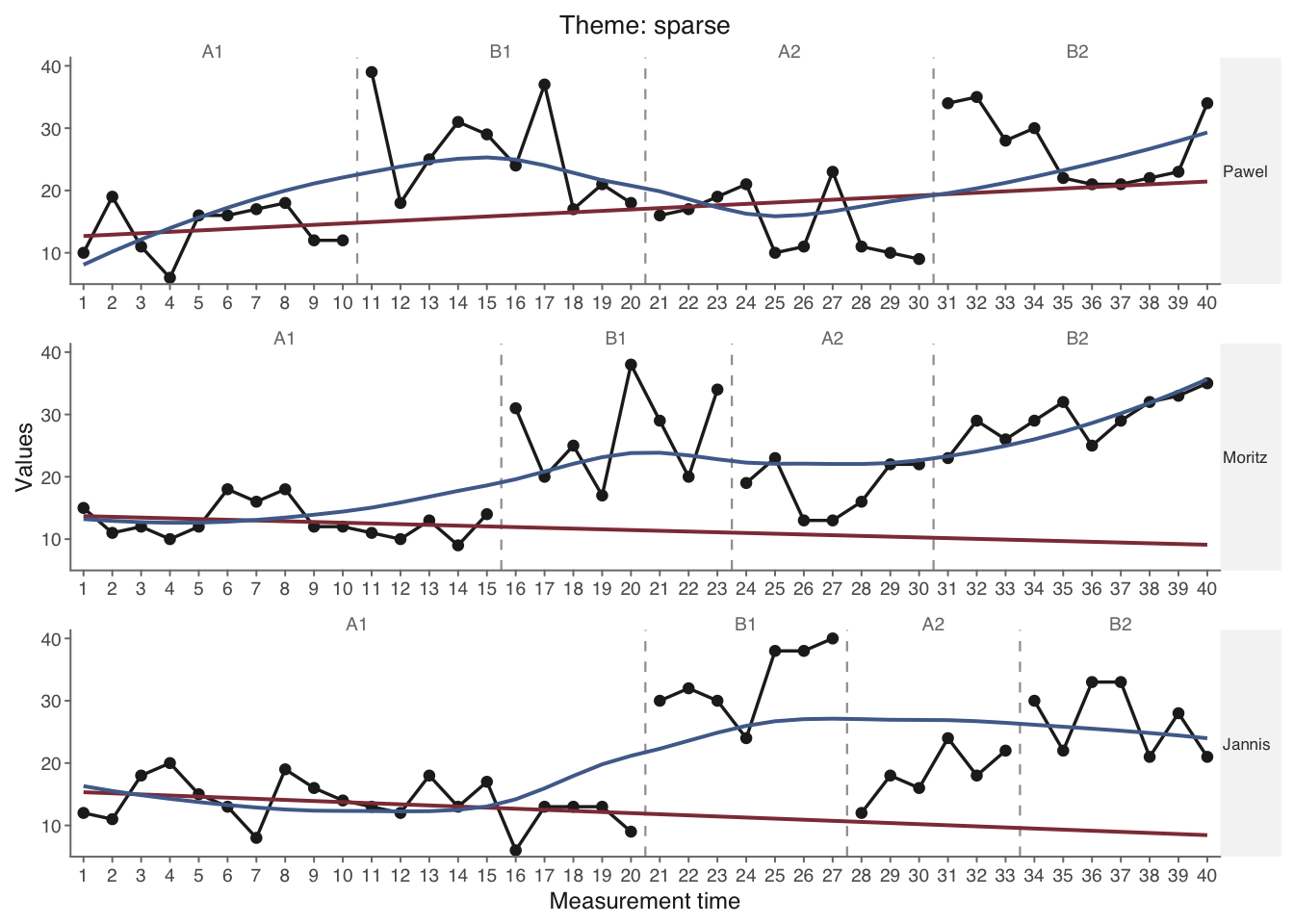
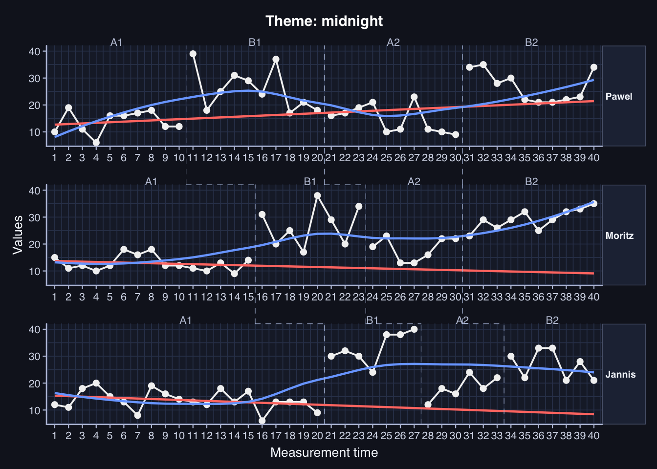
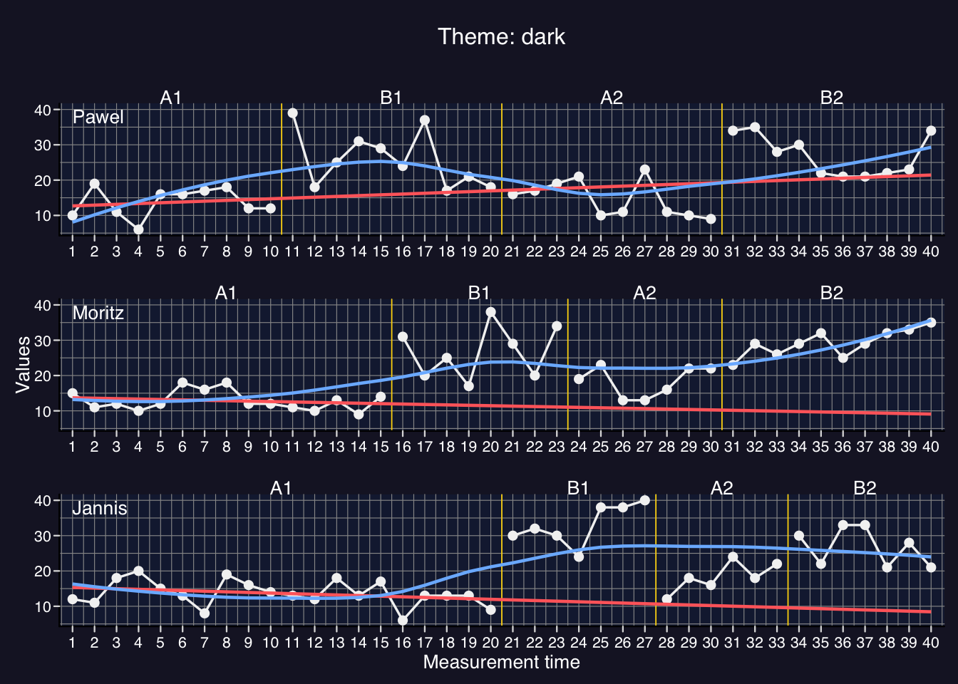
basic, colours_muted, colours_bw, colors_publication, colors_blind, colors_presentation, grid, grid2, grid3, small, tiny, big, phase_color, phase_shade, staircase, strip, minimal, dark, illustration, clarity, midnight, journal, playful, atelier, bauhaus, poster, handout, sparse, sienna

5.8.1 An overview

basic

minimal

illustration

clarity

journal

poster

handout

sparse

midnight

dark

playful

atelier

bauhaus

sienna

5.8.2 Combine themes

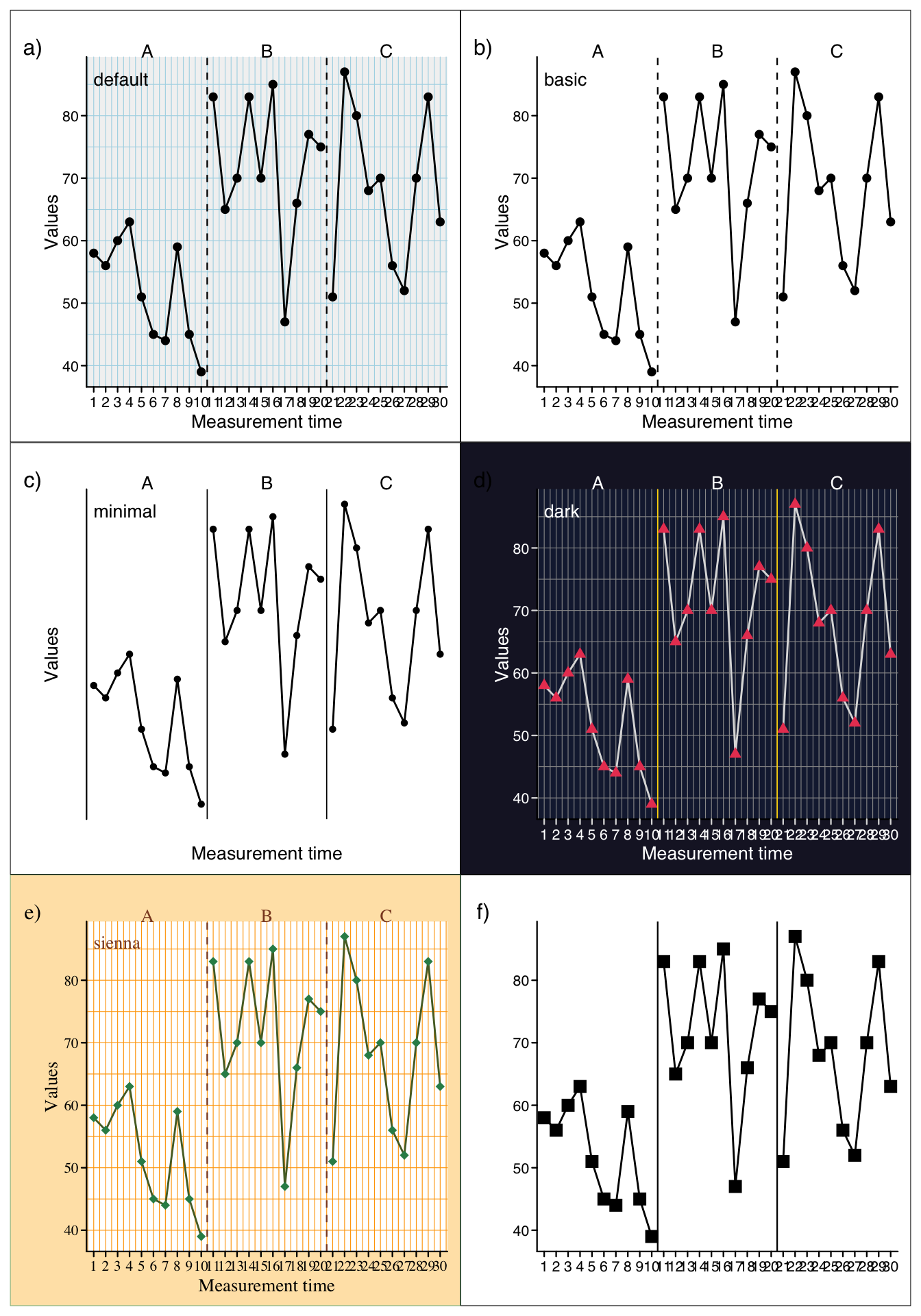
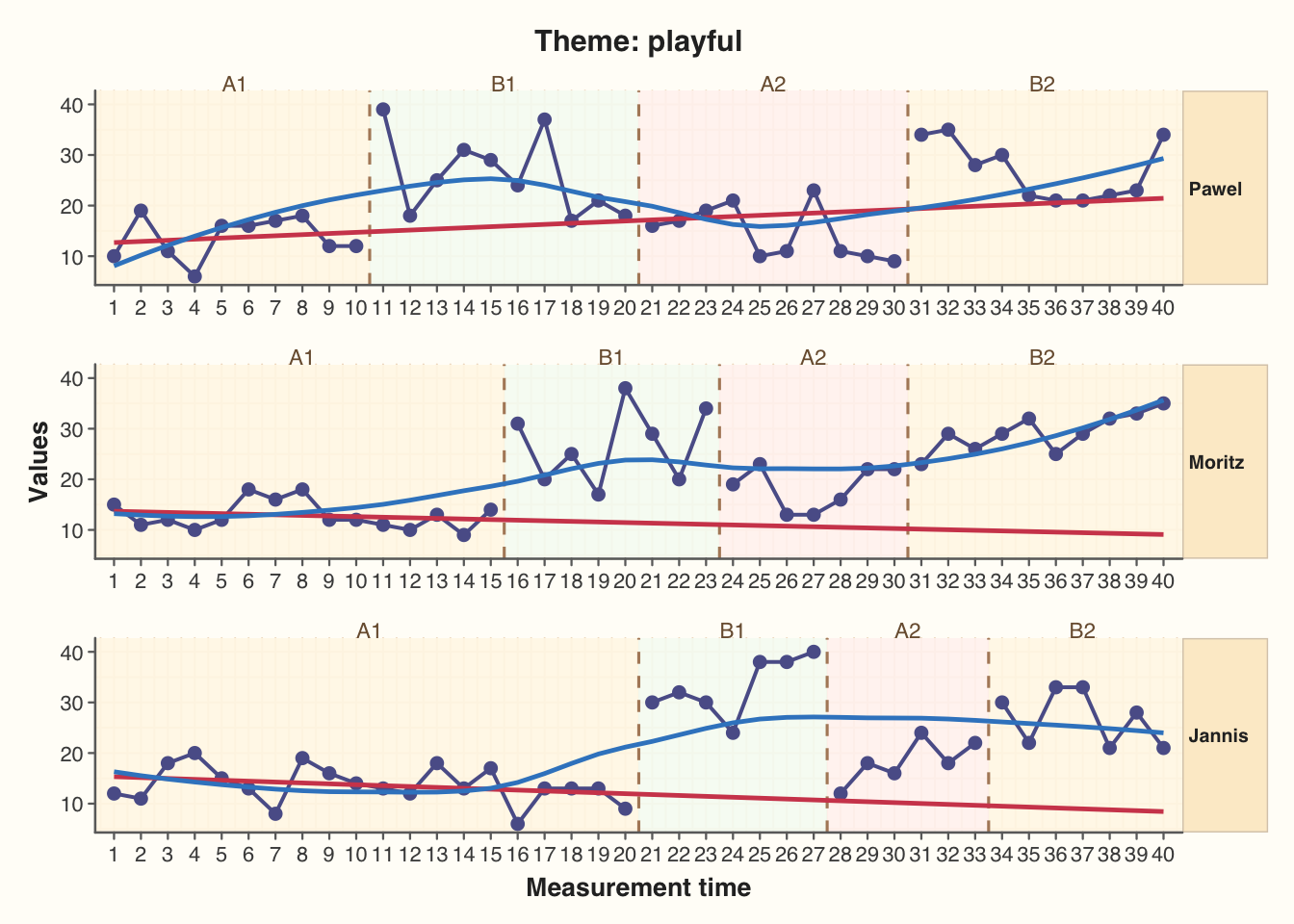
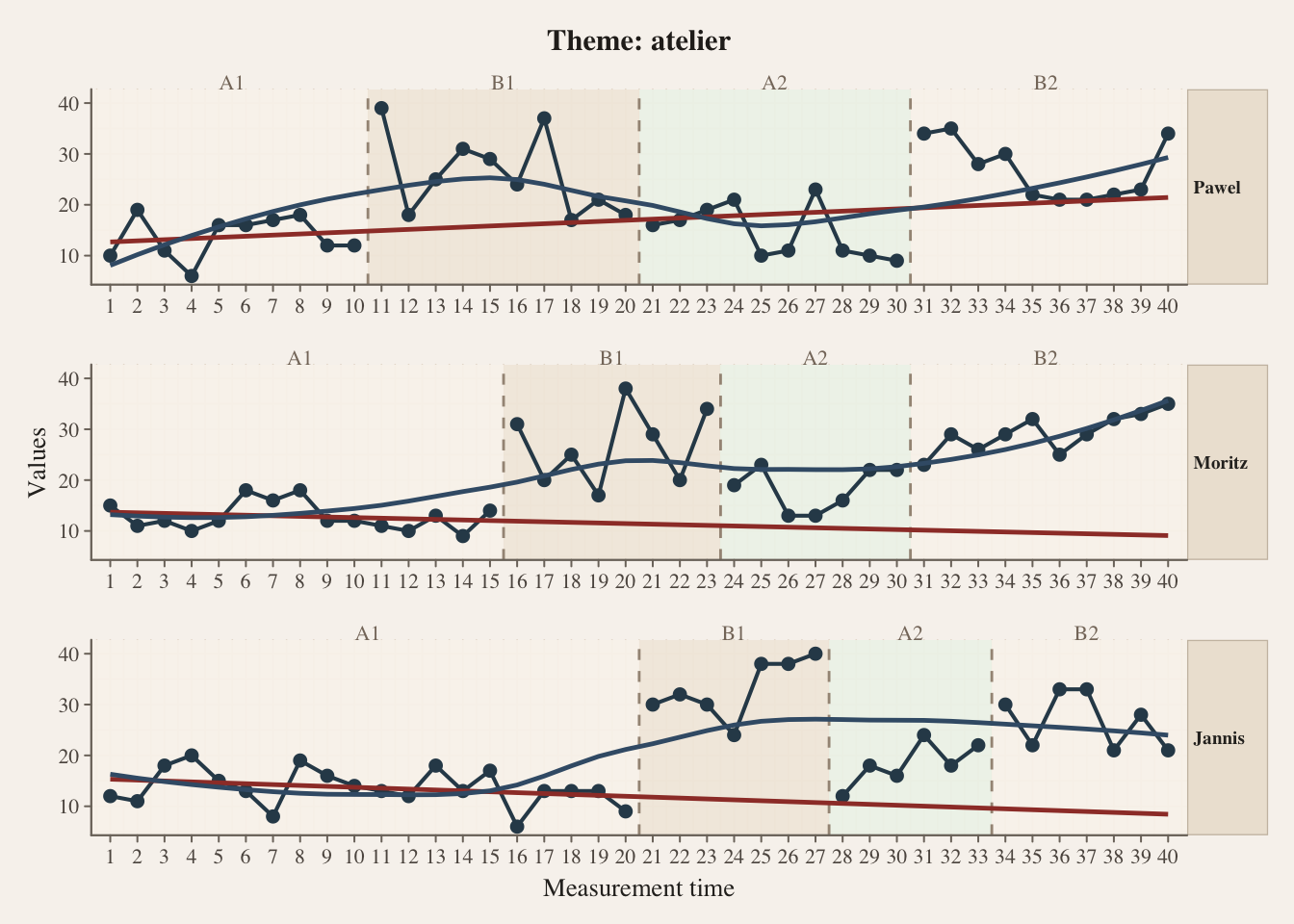
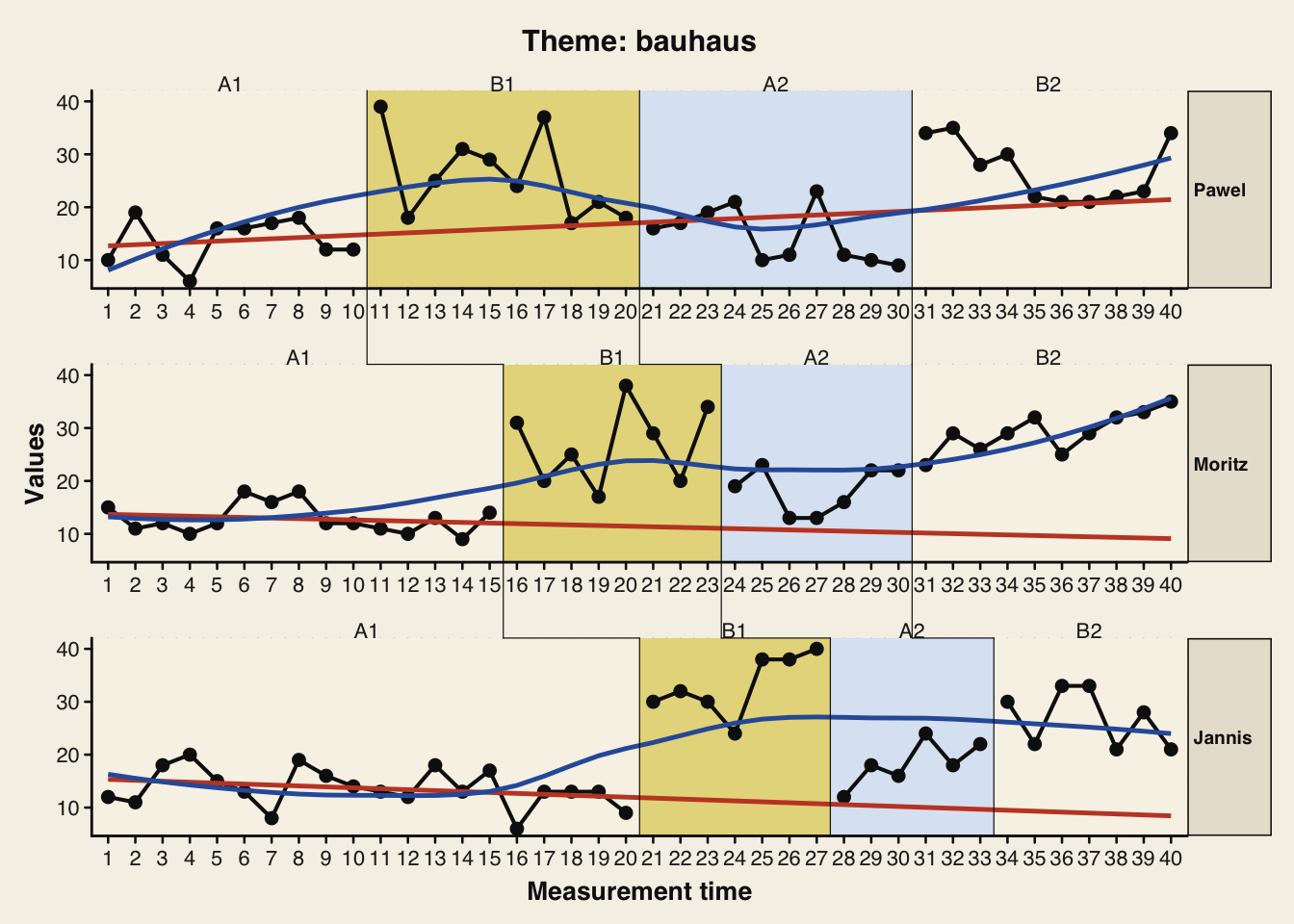
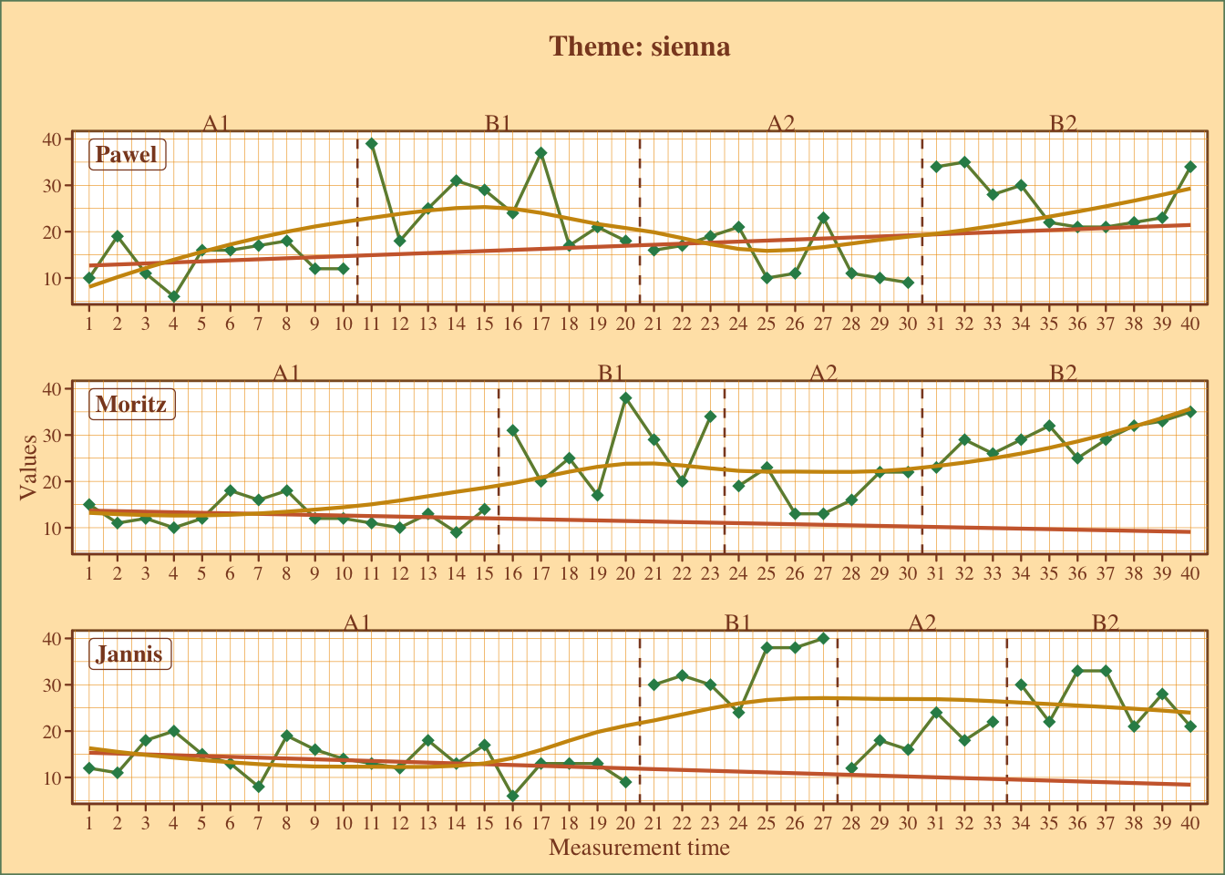
When providing multiple themes the order is important as the latter overwrites styles of the former.

scplot(exampleABC) |>
  set_theme("sienna", "minimal", "small", "phase_color")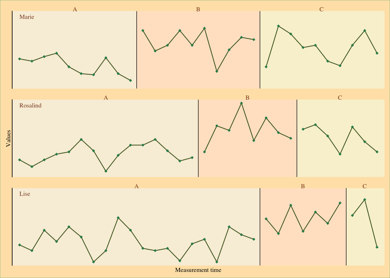

5.8.3 Create custom themes

For creating a custom theme, start with the new_theme() function and add all styling parameters like described above. The resulting new object can now be applied to the set_theme() function:

my_theme <- new_theme() |>
  set_panel(color = "red")  |>
  set_base_text(size = 12, color = "blue")  |>
  set_dataline(color = "darkred", linewidth = 2)

scplot(exampleABC)  |> set_theme(my_theme)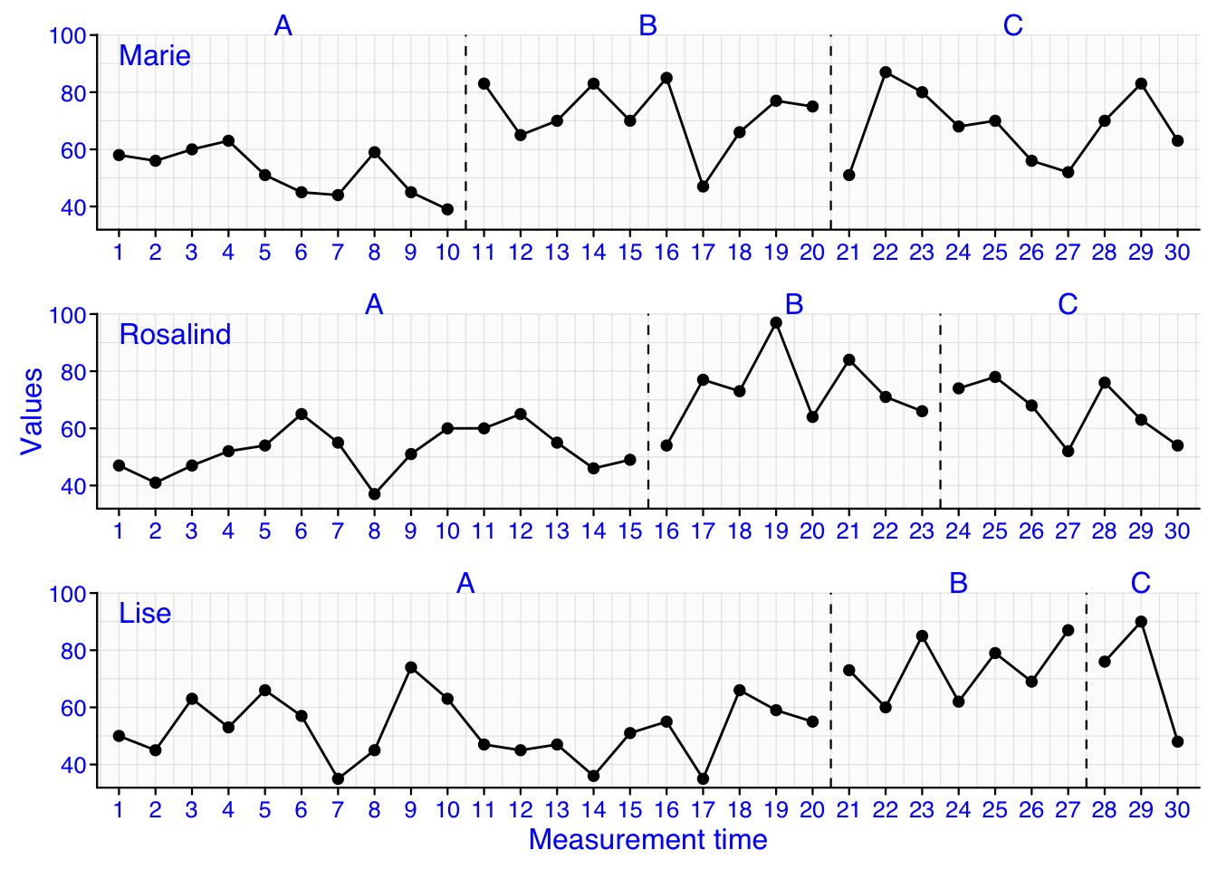

5.9 Set base text

The base text size is the absolute size. All other text sizes are relative to this base text size.

scplot(exampleAB_decreasing$Peter) |>
  set_base_text(colour = "blue", family = "serif", face = "italic", size = 14)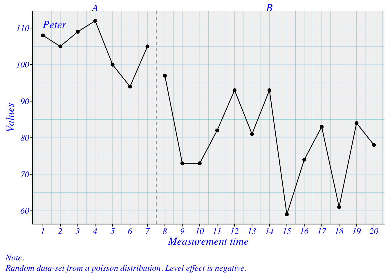

5.10 Add title and caption

scplot(exampleAB_decreasing) |>
  add_title("A new plot", color = "darkblue", size = 1.3) |>
  add_caption("Note. What a nice plot!", face = "italic", color = "darkred")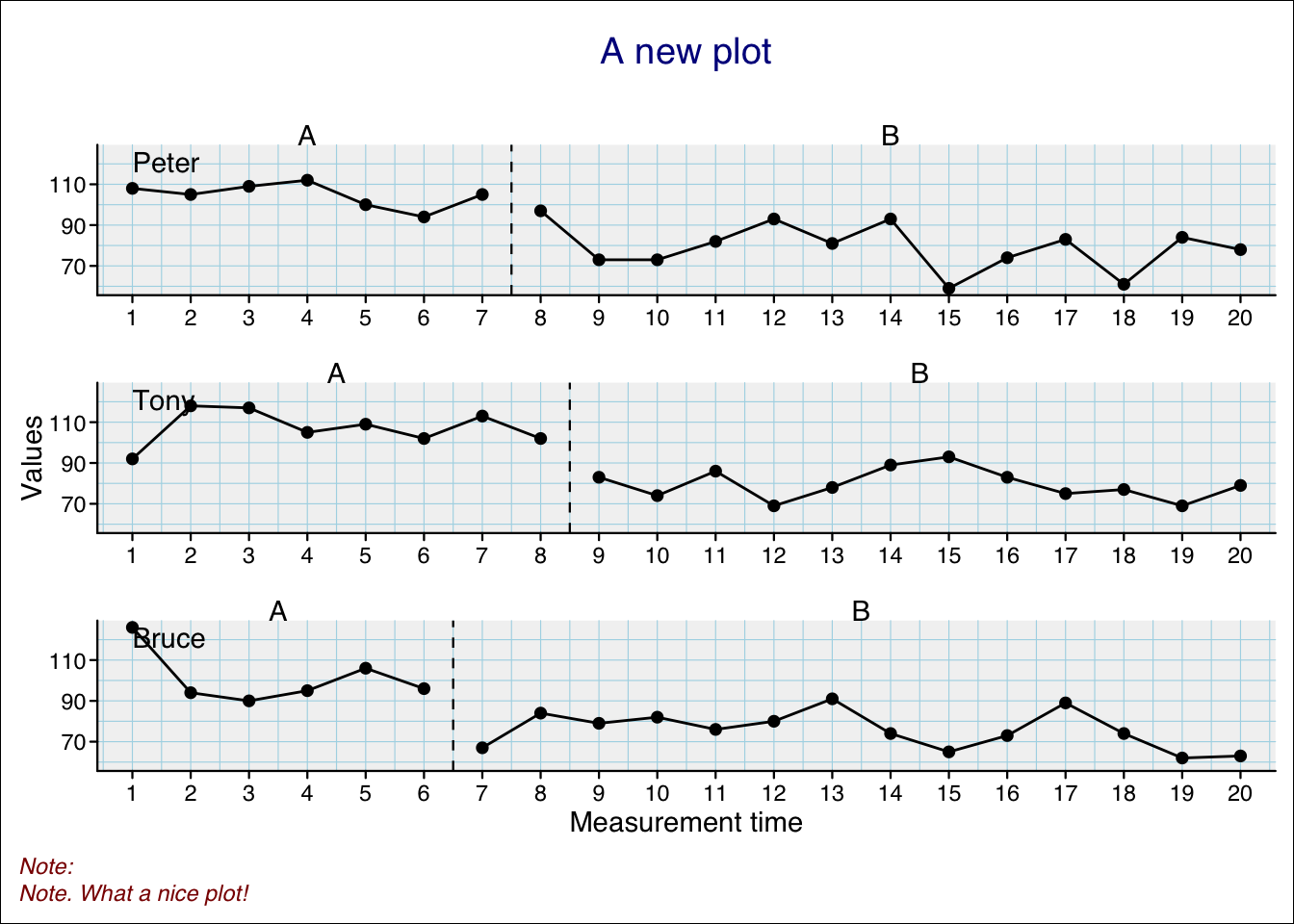

5.11 Add a legend

The add_legend() function adds a predefined legend that includes all datalines and statlines you have added. The labels for these lines are set automatically if you did not set the label argument in the corresponding set_dataline() and add_statline() functions.

Here is a simple example:

scplot(exampleABC) |>
  add_statline("mean", color = "darkred") |>
  add_statline("min", phase = "B", linewidth = 0.2, color = "darkblue") |>
  add_legend()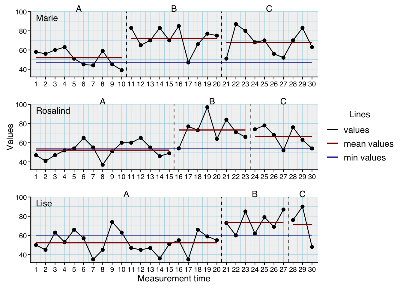

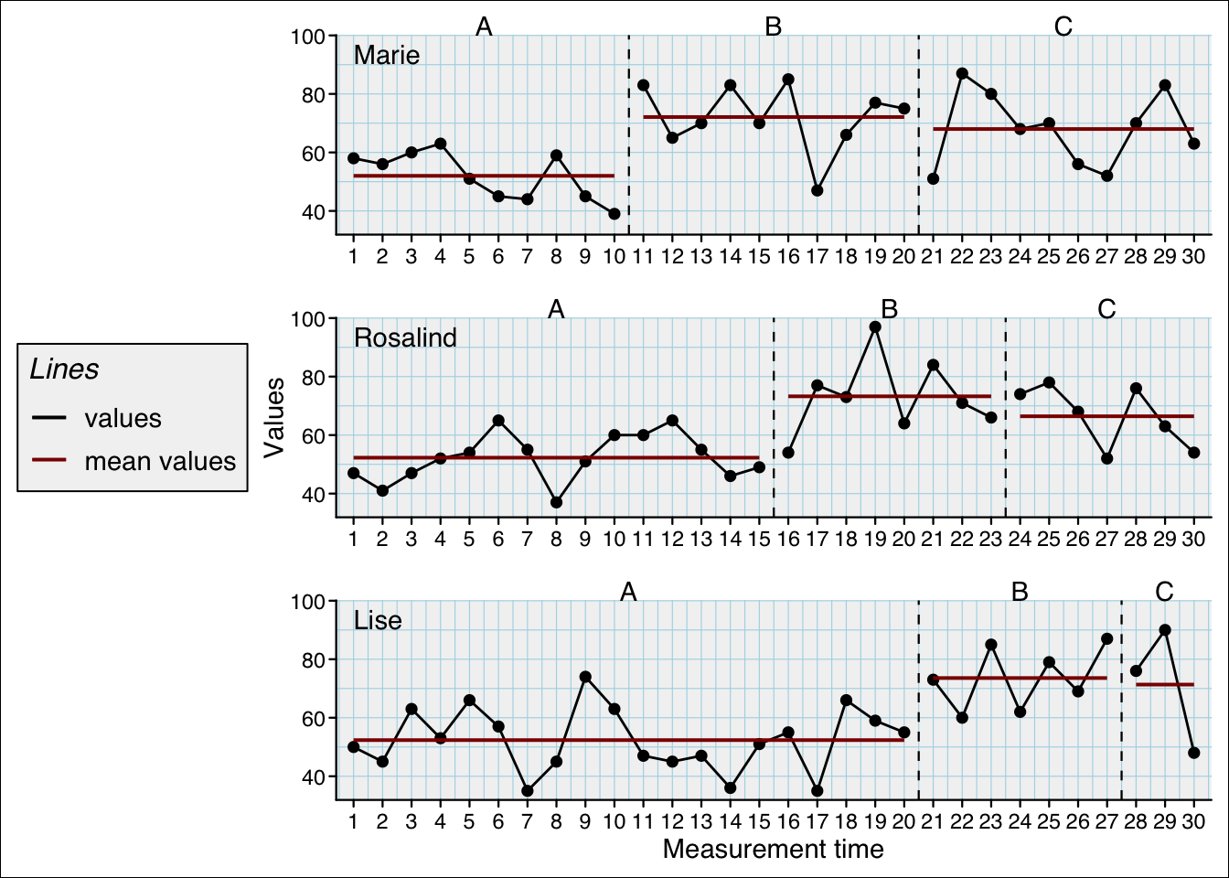
And here is a more advanced example that uses several arguments to defines the style of the legend:

scplot(exampleAB_add) |>
  set_dataline(label = "Pychological Wellbeing") |>
  set_dataline(variable = "depression", color = "darkblue", label = "Depression") |>
  add_statline(stat = "mean", label = "Wellbeing mean") |>
  add_statline(stat = "mean", variable = "depression", label = "Depression mean") |>
  set_phasenames(position = "none") |>
  set_panel(fill = c("lightblue", "grey80")) |>
  add_legend(
    position = "left",
    section_labels = c("Variables", "Section"),
    title = list(color = "brown", size = 10, face = 2),
    text = list(color = "darkgreen", size = 10, face = 2),
    background = list(color = "lightgrey")
  )

5.12 Axis settings

When axis ticks are to close together set the increment argument to leave additional space (e.g. increment = 2 will annotate every other value). When you set increment_from = 0 an additional tick will be set at 1 although counting of the increments will start at 0.

scplot(exampleA1B1A2B2) |> 
  set_xaxis(increment_from = 0, increment = 5, 
            color = "darkred", size = 0.7, angle = -90) |>
  set_yaxis(limits = c(0, 50), size = 0.7, color = "darkred")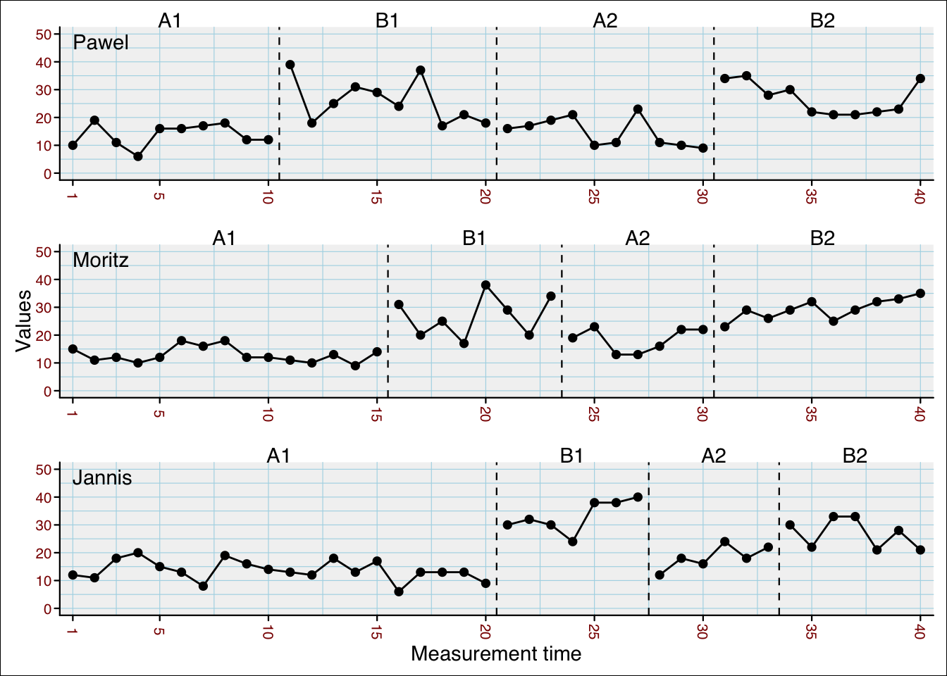 

5.13 Axis labels

scplot(exampleA1B1A2B2) |> 
  set_ylabel("Score", color = "darkred", angle = 0) |>
  set_xlabel("Session", color = "darkred")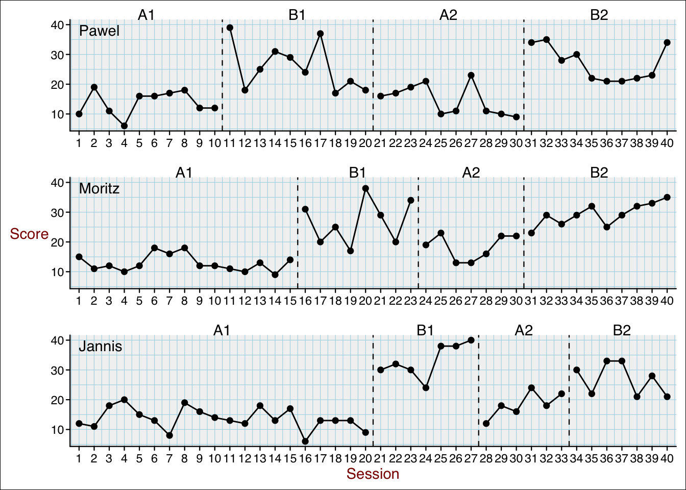

5.14 Change Casenames

scplot(exampleA1B1A2B2) |>
  set_casenames(c("A", "B", "C"), color = "darkblue", size = 1)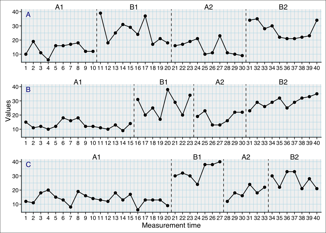

Casenames as strips:

scplot(exampleA1B1A2B2) |>
  set_casenames(position = "strip", 
                background = list(fill = "lightblue"))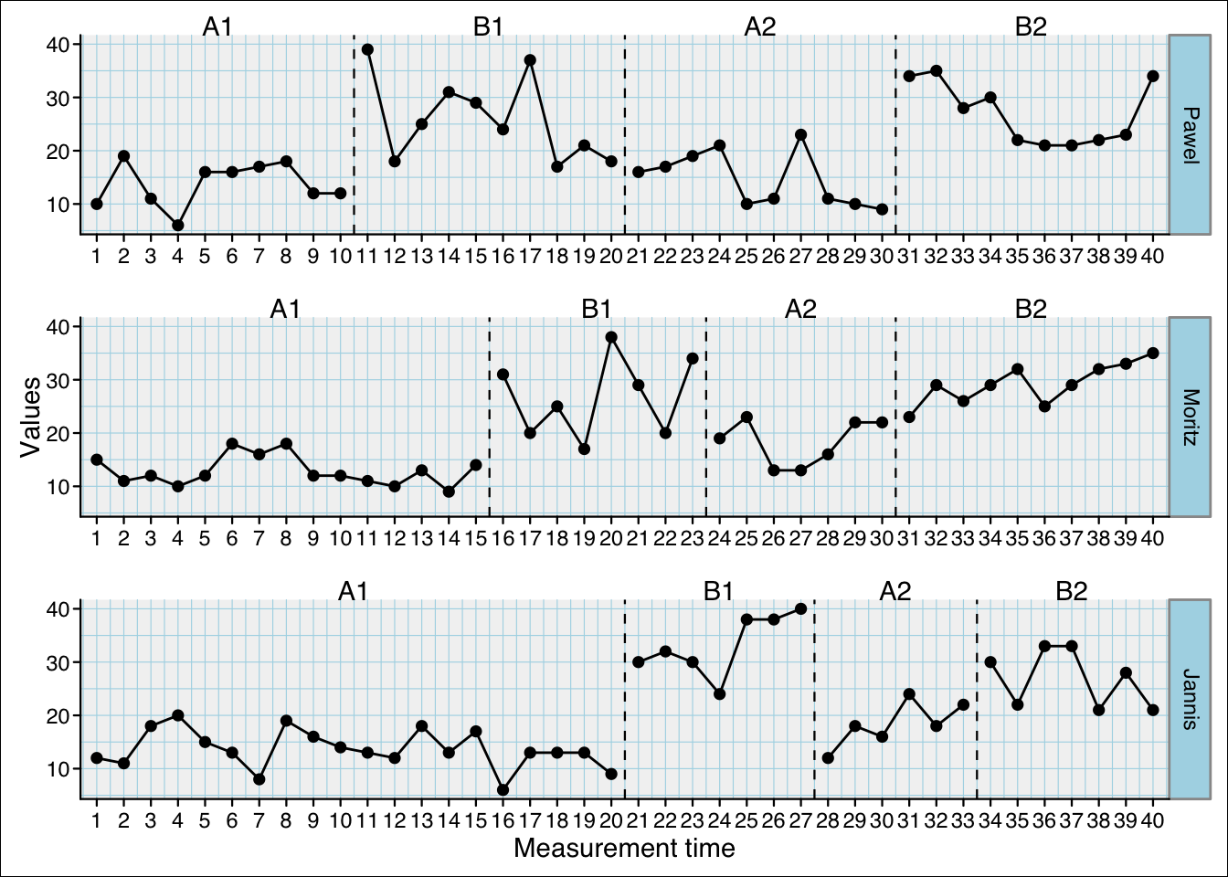

5.15 Add value labels

TipThe add_labels function call:

add_labels(
  object,
  nudge_y = 5,
  nudge_x = 0,
  round = NULL,
  text = list(),
  background = list(),
  variable = “.dvar”,
  padding = NULL
)

This function adds value labels to each data point. By deafult, the labels are placed above the data points. This can be changed with the nudge_y and nudge_x arguments (e.g., nudge_y = 7 will nudge the labels 7 units above the data points). A round argument can be used to round the values. The text and background of the labels can be styled with the text and background arguments which take a list with styling arguments. The padding argument sets the space between the text and the background of the label. Here is an example with the labels nudged above the data points:

scplot(exampleABC) |> 
  add_labels(text = list(color = "black", size = 0.7), 
             background = list(fill = "grey98"), nudge_y = 7)

Warning: Removed 1 row containing missing values or values outside the scale range
(`geom_label()`).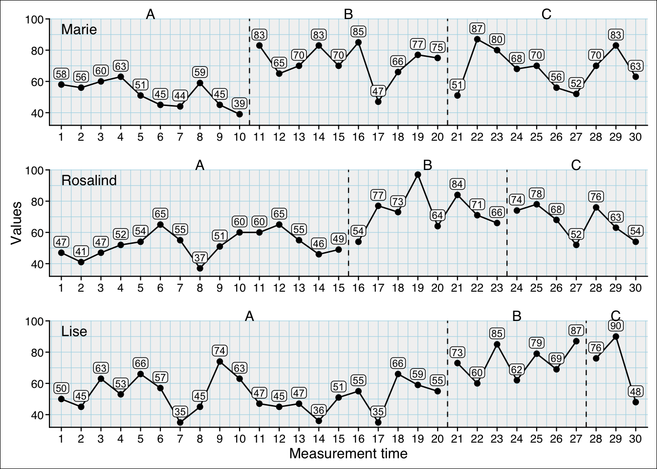

If you set the nudge_y argument to 0, the label will be set on-top the datapoints:

scplot(exampleABC) |> 
  set_theme("minimal") |>
  add_labels(text = list(color = "black", size = 0.7), 
             background = list(fill = "grey98"), 
             nudge_y = 0, padding = 0.25)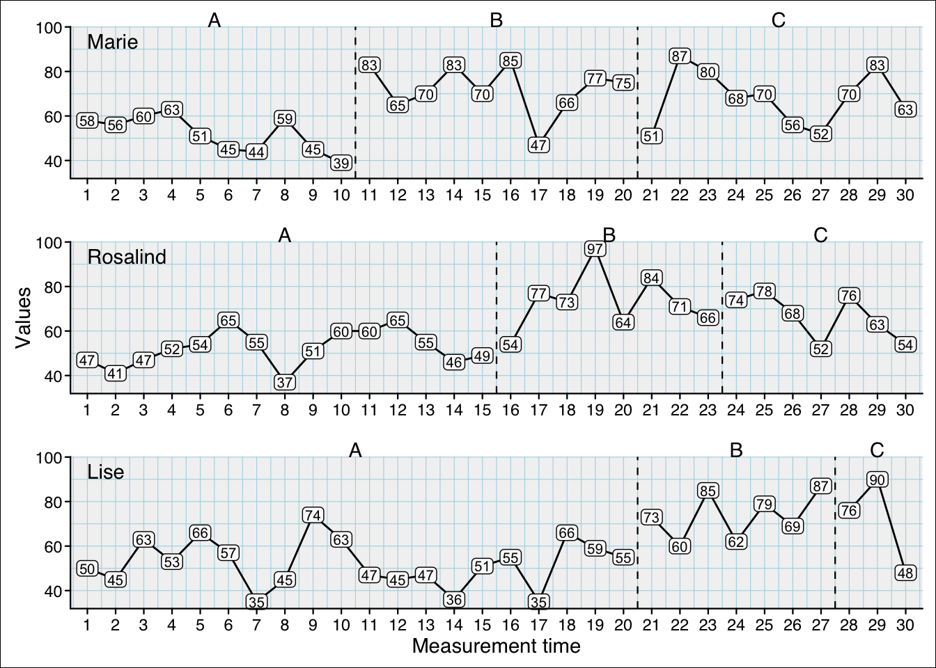

5.16 Add a ridge

Adds a ridge element to an scplot object. Ridges mark the area below the dataline. The colour of the ridge is set by the color argument. The argument variable can be used to specify which dataline the ridge should be based on. If not specified, the default dataline will be used.

scplot(exampleAB_mpd) |> 
  add_ridge("grey50")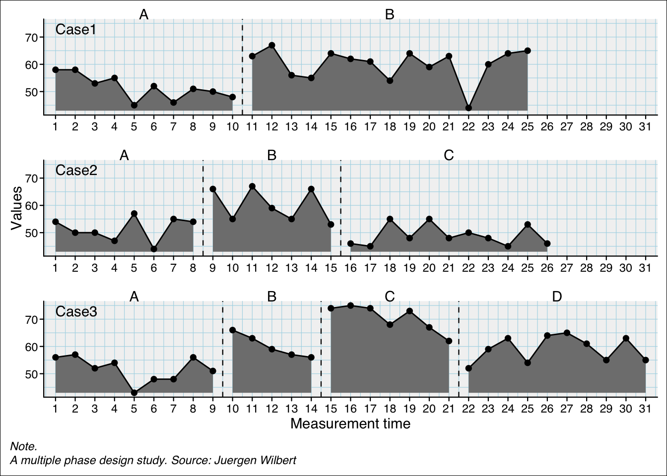

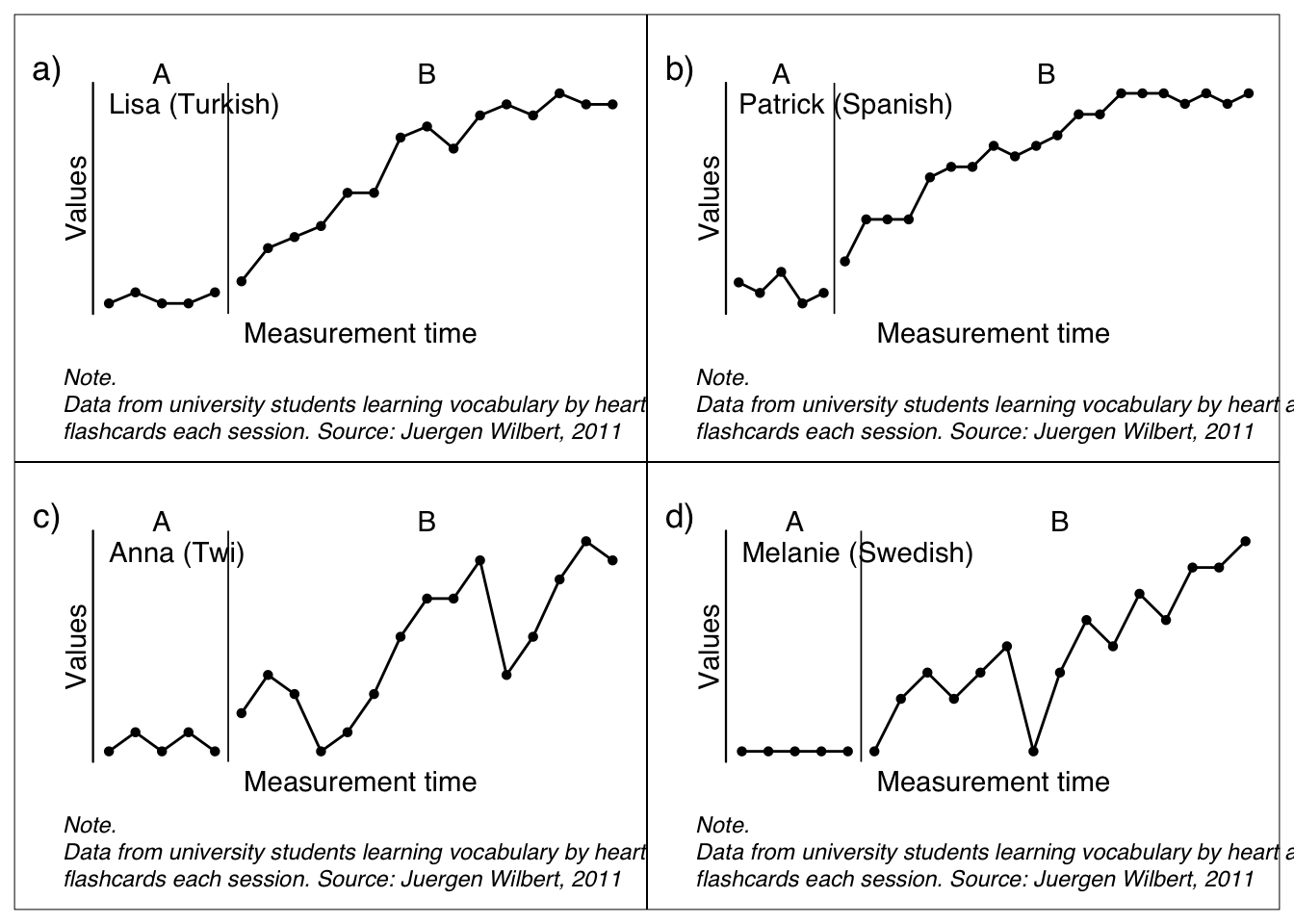
5.17 Extending scplot with ggplot2

scplot() generates ggplot2 objects. You can keep the ggplot2 object and assign it into a new object with the as_ggplot() function. Thereby, you can use many ggplot2 functions to rework your graphics:

# remove caption and apply a new default theme for all following scplots
options(scplot.plot.caption = NULL, 
        scplot.plot.theme = c("basic","minimal"))

# rename cases
names(byHeart2011) <- c("Lisa", "Pat", "Anna", "Lena")

# create ggplot objects for each case
p1 <- scplot(byHeart2011[1]) |> as_ggplot()
p2 <- scplot(byHeart2011[2]) |> as_ggplot()
p3 <- scplot(byHeart2011[3]) |> as_ggplot()
p4 <- scplot(byHeart2011[4]) |> as_ggplot()

# combine the ggplot objects with patchwork and add a title
library(patchwork)
p1 + p2 + p3 + p4 + plot_annotation(
  tag_levels = "a", tag_suffix =  ")",
  title = "Data from university students learning vocabulary by heart"
)

options(scplot.plot.caption = "auto", scplot.plot.theme = "default")

5.18 Complexs examples

Here are some more complex examples

scplot(example_A24) |> 
  add_statline("lowess", linewidth = 1.5) |>
  add_statline("loess", linewidth = 1.5) |>
  add_statline("moving mean", lag = 3, linewidth = 1.5) |>
  set_xaxis(size = 0.8, angle = 35) |>
  set_dataline(point = "none") |>
  add_legend(position = c(0.8, 0.75), background = list(color = "grey50")) |>
  set_phasenames(c("no speedlimit", "with speedlimit"), 
                 position = "left", hjust = 0, vjust = 1) |>
  set_casenames(position = "none") |>
  add_title("Effect of a speedlimit on the A24") |>
  add_caption("Moving mean calculated with lag three", face = 3, size = 1) |>
  add_ridge(color = "lightblue")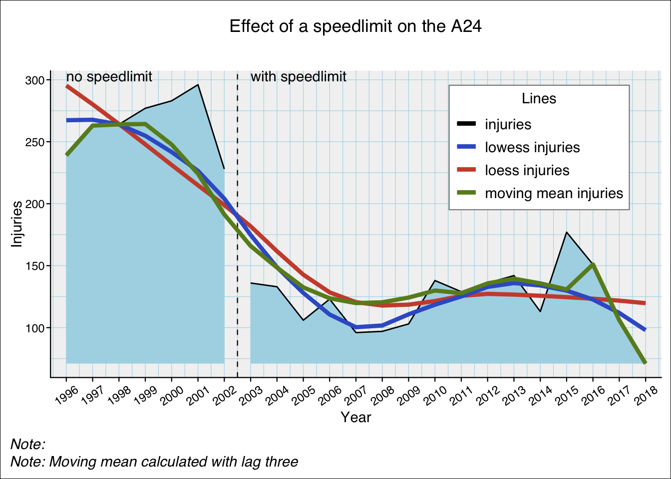

scplot(exampleAB_add) |>
  set_dataline("cigarrets", point = list(size = 1)) |>
  add_statline("trend", linetype = "dashed", label = "Trend of wellbeing") |>
  add_statline("mean", variable = "cigarrets", color = "darkred", label = "Mean of cigarrets") |>
  add_marks(positions = c(14,20), size = 3, variable = "cigarrets")|>
  add_marks(positions = "cigarrets > quantile(cigarrets, 0.75)", size = 3) |>
  set_xaxis(increment = 5) |>
  set_phasenames(color = NA) |>
  set_casenames(position = "strip") |>
  add_legend(
    section_labels = c("", ""),
    text = list(face = 3)
  ) |>
  set_panel(fill = c("lightblue", "grey80")) |>
  add_ridge(color = "snow", variable = "cigarrets") |>
  add_labels(variable = "cigarrets", nudge_y = 2, 
             text = list(color = "blue", size = 0.5)) |>
  add_labels(nudge_y = 2, text = list(color = "black", size = 0.5),
             background = list(fill = "white"))

Warning: Removed 1 row containing missing values or values outside the scale range
(`geom_label()`).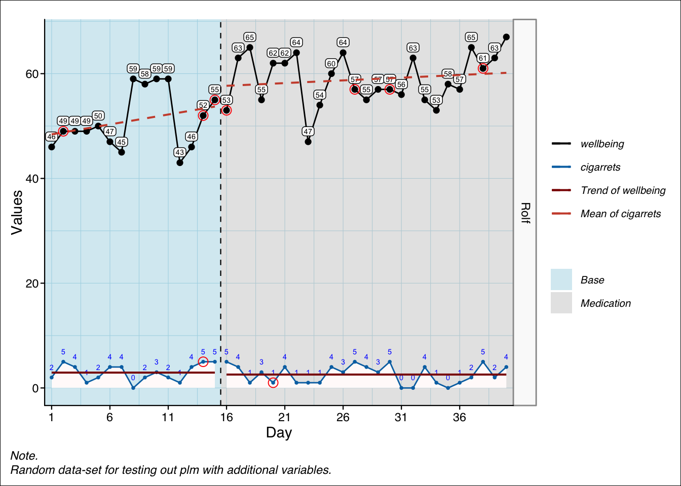

scplot(exampleA1B1A2B2) |> 
  set_xaxis(increment = 4, size = 0.7) |>
  set_yaxis(color = "sienna3") |>
  set_ylabel("Points", color = "sienna3", angle = 0) |>
  set_xlabel("Weeks", size = 1, color = "brown") |>
  add_title("Points by week", color = "sienna4", face = 3) |>
  add_caption("An extensive Example.",
              color = "black", size = 1, face = 3) |>
  set_phasenames(c("Baseline", "Intervention", "Fall-Back", "Intervention_2"), 
                 size = 0) |>
  add_ridge(scales::alpha("lightblue", 0.5)) |>
  set_casenames(labels = sample_names(3), color = "steelblue4", size = 0.7) |>
  set_panel(fill = c("grey80", "grey95"), color = "sienna4") |>
  add_grid(color = "grey85", linewidth = 0.1) |>
  set_dataline(linewidth = 0.5, linetype = "solid", 
               point = list(colour = "sienna4", size = 0.5, shape = 18)) |>
  add_labels(text = list(color = "sienna", size = 0.7), nudge_y = 4) |>
  set_separator(linewidth = 0.5, linetype = "solid", color = "sienna") |>
  add_statline(stat = "trendA", color = "tomato2") |>
  add_statline(stat = "max", phase = c(1, 3), linetype = "dashed") |>
  add_marks(case = 1:2, positions = 14, color = "red3", size = 2, shape = 4) |>
  add_marks(case = "all", positions = "values < quantile(values, 0.1)", 
            color = "blue3", size = 1.5) |>
  add_marks(positions = outlier(exampleABAB), color = "brown", size = 2) |>
  add_text(case = 1, x = 5, y = 35, label = "Interesting", 
           color = "darkgreen", angle = 20, size = 0.7) |>
  add_arrow(case = 1, 5, 30, 5, 22, color = "steelblue") |>
  set_background(fill = "white") |>
  add_legend() |>
  set_theme("basic") |>
  set_theme_element(panel.spacing.y = unit(0, "points"))

Warning: Removed 6 rows containing missing values or values outside the scale range
(`geom_text()`).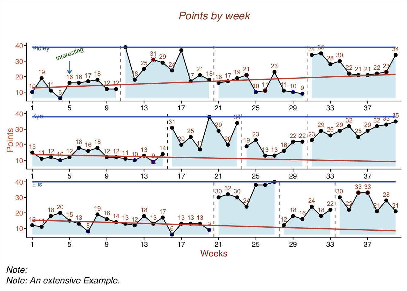

5.19 Experimental features

Some features are still experimental and might change in future versions. They are not included in the documentation yet but you can already try them out.

5.19.1 Staircase style separators

scplot(exampleABC) |>
  set_separator(staircase = TRUE, color = "darkred", linetype = "solid", linewidth = 1.5)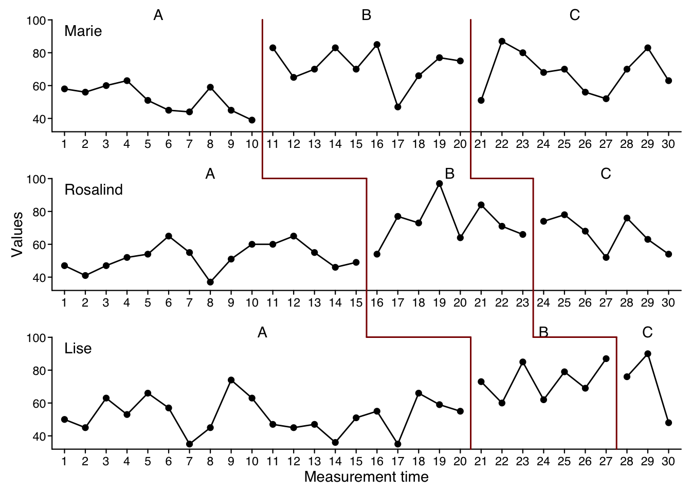

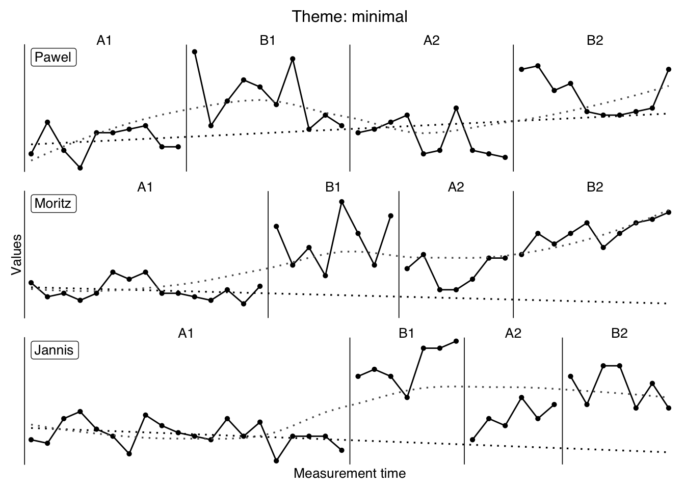
scplot(exampleA1B1A2B2) |> 
  set_theme("minimal", "tiny", "staircase")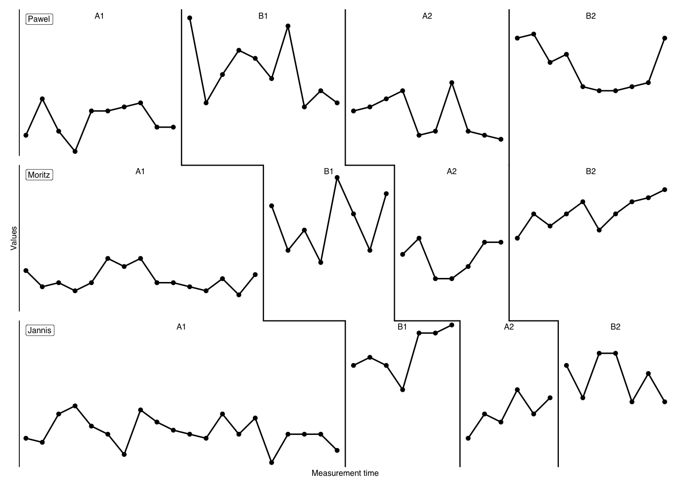

5.19.2 Alternating treatment design

scplot(scan::example_atd) |> 
  split_dataline("treatment") |> 
  add_legend()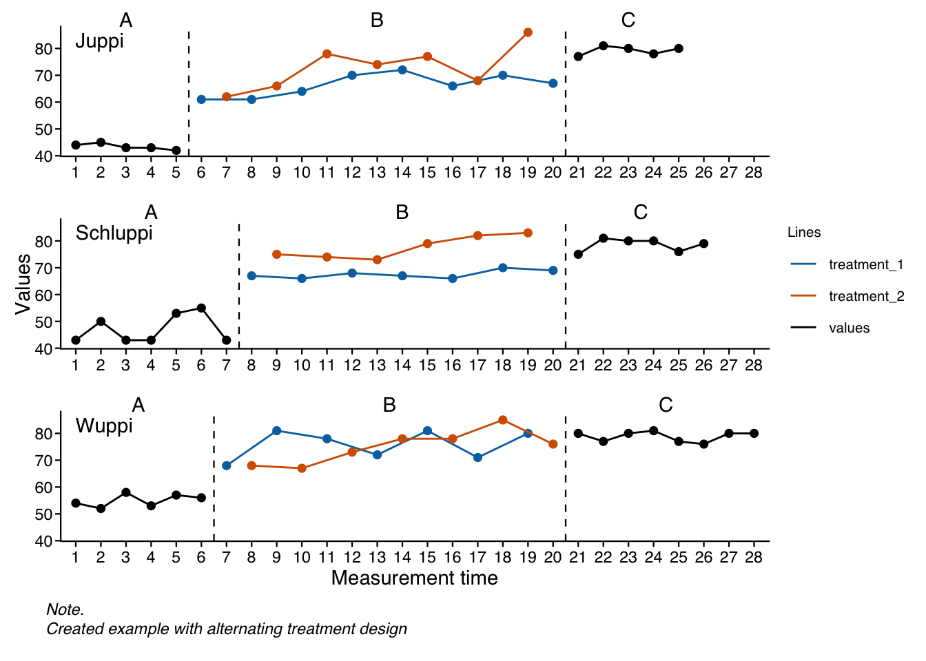

scplot(scan::example_atd) |> 
  split_dataline("treatment", labels = c("Maze", "PGC")) |> 
  add_legend()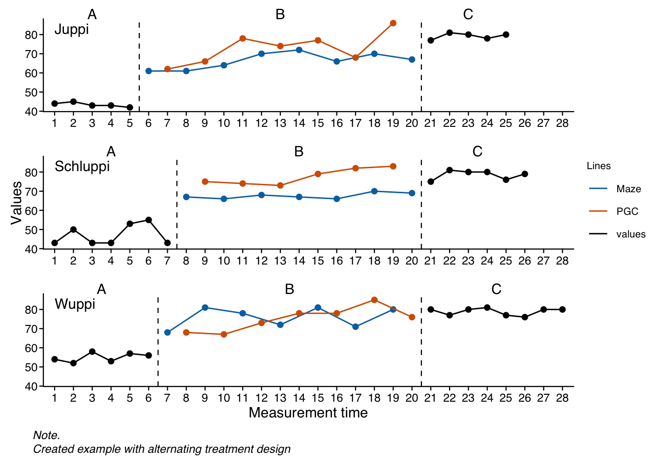

5.19.3 Adding bars

• Set the type argument to "bar"
  
• Extend the limits of the x-axis by 1 (here from 0 to 41)
  
• Set the left margin of the x-axis to 0 with the expand argument.

scplot(exampleAB_add) |>
  set_xaxis(expand = c(0, 0), limits = c(0, 41)) |>
  set_dataline("cigarrets", type = "bar", linewidth = 0.6, point = "none") |>
  add_statline("mean", variable = "cigarrets", color = "darkred") |>
  add_statline("trend", linetype = "dashed") |>
  set_casenames(position = "strip")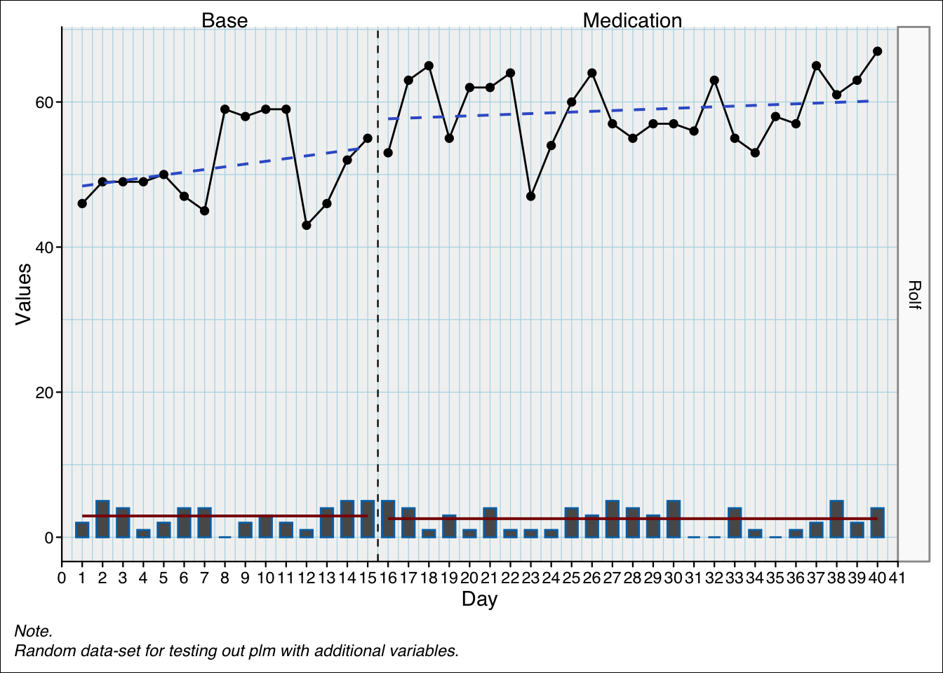

---

1. It replaces the plot.scdf() (or: plotSC()) function already included in scan (see Section D.1). For the time being, the “old” plot.scdf will be kept in future versions of scan.

2. with install.packages("scplot")