10  Piecewise linear regressions

In a piecewise-regression analysis (sometimes called segmented regression) a dataset is split at a particular break point and the regression parameters (intercept and slopes) are calculated separately for the data before and after the break point. This is done because we assume that there is a qualitative change at the break point that affects the intercept and slope. This approach is well suited to the analysis of single-case data which are from a statistical point of view time-series data segmented into phases. A general model for single-case data based on the piecewise regression approach has been proposed by Huitema and McKean Huitema & Mckean (2000). They refer to two-phase single-case designs with a pre-intervention phase containing some measurements before the start of the intervention (A-phase) and an intervention phase containing measurements starting at the beginning of the intervention and continuing throughout intervention (B-phase).

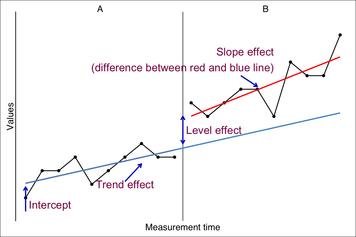
In this model, four parameters predict the outcome at a specific measurement point see 10.1

1. The performance at the beginning of the study (intercept),

2. a developmental effect leading to a continuous increase throughout all measurements (trend effect),

3. an intervention effect leading to an immediate and constant increase in performance (level effect), and

4. a second intervention effect that evolves continuously with the beginning of the intervention (slope effect).

Figure 10.1: Illustration of the piecewise-linear model

The regression model

The default model applied in the plm function has the formula

\[ y_i = \beta_0 + \beta_1 (time_i-time_1) + \beta_2 phase_i + \beta_3 (time_i-time_{n_A+1})*phase_i \]

Where:

\(i\) := the session¹ number.

\(\beta_0\) := the intercept.

\(\beta_1 time\) := the continuous effect of the measurement time (the trend effect).

\(\beta_2 phase\) := the discrete effect of the phase switch (the level effect).

\(\beta_3 (time-n_{A+1})*phase\) := the continuous effect of the phase switch (the slope effect).

\(n_{A+1}\) := the first session of phase B.

For \(\beta_1\) and \(\beta_3\), the time variables are shifted to start with a 0 at the first session of the respective phase.

scan provides an implementation based on this piecewise-regression approach. Though the original model is extended by several factors:

• multiple phase designs
• additional (control) variables
• autoregression modelling
• logistic, binomial, and poisson distributed dependent variables and error terms
• multivariate analyses for analysing the effect of an intervention on more than one outcome variable (see Chapter 12).
• multilevel analyses for multiple cases (see Chapter 11).

10.1 The basic plm function

The plm function call

plm(data, dvar, pvar, mvar, AR = 0, model = c(“W”, “H-M”, “B&L-B”, “JW”), family = “gaussian”, trend = TRUE, level = TRUE, slope = TRUE, contrast = c(“first”, “preceding”), contrast_level = c(NA, “first”, “preceding”), contrast_slope = c(NA, “first”, “preceding”), formula = NULL, update = NULL, na.action = na.omit, r_squared = TRUE, var_trials = NULL, dvar_percentage = FALSE, …)

The basic function for applying a regression analyses to a single-case dataset is plm. This function analyses one single-case. In its simplest way, plm takes one argument with an scdf object and it returns a full piecewise-regression analyses.

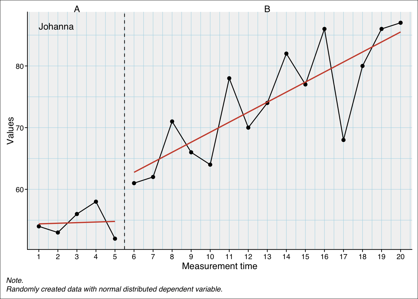
plm(exampleAB$Johanna)

Piecewise Regression Analysis

Contrast model: W / level = first, slope = first

Fitted a gaussian distribution.
F(3, 16) = 28.69; p = 0.000; R² = 0.843; Adjusted R² = 0.814; AIC = 126.8444

                            B LL-CI95% UL-CI95%    SE      t     p delta R²
Intercept              54.400   46.776   62.024 3.890 13.986 0.000         
Trend (mt)              0.100   -3.012    3.212 1.588  0.063 0.951    0.000
Level phase B (phaseB)  7.858   -3.542   19.258 5.816  1.351 0.195    0.018
Slope phase B (interB)  1.525   -1.642    4.692 1.616  0.944 0.359    0.009

Autocorrelations of the residuals
 lag    cr
   1 -0.32
   2 -0.13
   3 -0.01
Ljung-Box test: X²(3) = 2.84; p = 0.417 

Formula: values ~ 1 + mt + phaseB + interB 

The output shows the specific contrast settings for the phase and slope calculation (see below for a detailed explanation). Next, the overall model fit is provided. In this specific example the model fit is quite high explaining more than 80% of the variance of the dependent variable. The following regression table shows the unstandardised estimates (B), the lower and upper boundaries of a 95% confidence interval, the standard-error, the t-test statistic, the p-value, and the delta R squared for each predictor.

In this example, the intercept is the score estimation at the beginning of the study (here: at the first session, see Figure 10.2). The trend effect (variable mt) is 0.100. This means that for every one point increase in measurement-time, the score increased by 0.100. As this example has a total of 20 sessions, the overall increase due to the trend is \(19 * 0.100 = 1.9\) points. The level effect (variable phase with level B) is 7.858. This means that all scores of phase B are increased by 7.858 points. The slope effect (for phase B) is 1.525. This means that for every one point increase in measurement time after the first phase B session, the score increases by 1.525. As there are 15 Phase B sessions in this example, the total increase due to the slope effect is \(14 * 1.525 = 21.35\) points.

From these values each data point can be estimated. For example, the last session (\(i=20\)) is estimated to be \(54.400 + 19 * 0.100 + 7.858 + 14 * 1.525 = 85.508\).

scplot(exampleAB$Johanna) |> add_statline("trend")

Figure 10.2: Example dataset

Note

As a convenience, the predictors are renamed according to the respective effect within the single-case terminology that they represent.

If you prefer to use the original variable names, set the following option: options(scan.rename.predictors = "no").

If you want more concise renamed predictors, set: options(scan.rename.predictors = "concise").

You can restore the default renaming by setting: options(scan.rename.predictors = "full").

10.2 Autocorrelation of the residuals

The output also reports the autocorrelations of the residuals, which indicate whether the models residuals are serially independent.

There are many reasons why this might happen. For example, in a learning study, performance may temporarily decline after a learning session (performance dip). Similarly, in a medication study, a drug might initially cause a brief worsening of symptoms before exerting its intended therapeutic effect (early symptom exacerbation effect).

The lag refers to the number of measurement points between observations that show autocorrelation.

The Ljung-Box test is an omnibus test that evaluates whether the residuals exhibit significant autocorrelation at multiple lags. It assesses whether the joint distribution of autocorrelations differs significantly from what would be expected under the assumption of independence.

High and significant autocorrelations pose a threat to the validity of standard regression models, as they violate the assumption of independent residuals. To account for this, you can set the AR argument with the appropriate maximum lag (e.g., AR = 3). This implements an ARMA (autoregressive moving average) model, which takes the serial correlation in the residuals into account.

10.3 Standardizing predictors

If you want standardized predictors, meaning that predictors are scaled to standard deviations, the best approach is to standardize all variables before computing the regression model. Use the rescale() function to do this.

exampleAB$Johanna |> 
  rescale() |> 
  plm()

Rescaled values, mt

Piecewise Regression Analysis

Contrast model: W / level = first, slope = first

Fitted a gaussian distribution.
F(3, 16) = 28.69; p = 0.000; R² = 0.843; Adjusted R² = 0.814; AIC = 28.67075

                            B LL-CI95% UL-CI95%    SE      t     p delta R²
Intercept              -1.276   -1.931   -0.621 0.334 -3.818 0.002         
Trend (mt)              0.051   -1.531    1.633 0.807  0.063 0.951    0.000
Level phase B (phaseB)  0.675   -0.304    1.655 0.500  1.351 0.195    0.018
Slope phase B (interB)  0.775   -0.835    2.385 0.821  0.944 0.359    0.009

Autocorrelations of the residuals
 lag    cr
   1 -0.32
   2 -0.13
   3 -0.01
Ljung-Box test: X²(3) = 2.84; p = 0.417 

Formula: values ~ 1 + mt + phaseB + interB 

The regression coefficients B are now standardized Beta (ß) coefficients, indicating the expected change (in standard deviations) of the dependent variable for a one-standard-deviation increase in the predictor.

10.4 Adjusting the model

The plm model is a complex model specifically suited for single-case studies. It entails a series of important parameters. Nevertheless, often we have specific theoretical assumption that do no include some of these parameters. We might, for example, only expect an immediate but not a continuous change from a medical intervention. Therefore, it would not be useful to include the slope-effect into our modelling. Vice versa, we could investigate an intervention that will just develop across time without an immediate change with the intervention start. Here we should drop the level-effect from out model. Even the assumption of a trend-effect can be dropped in cases where we do not expect a serial dependency of the data and we do not assume intervention independent changes within the time-frame of the study.

It is important to keep in mind, that an overly complex model might have negative effects on the test power of an analyses (that is, the probability of detecting an actually existing effect is diminished) (see Wilbert, Lüke, & Börnert-Ringleb, 2022)

10.4.1 The slope, level, and trend arguments

The plm function comes with three arguments (slope, level, and trend) to include or drop the respective predictors from the plm model. Buy default, all arguments are set TRUE and a full plm model is applied to the data.

Consider the following data example:

example <- scdf(
   values = c(A = 55, 58, 53, 50, 52, 
              B = 55, 68, 68, 81, 67, 78, 73, 72, 78, 81, 78, 71, 85, 80, 76)
)

plm(example)

Piecewise Regression Analysis

Contrast model: W / level = first, slope = first

Fitted a gaussian distribution.
F(3, 16) = 21.36; p = 0.000; R² = 0.800; Adjusted R² = 0.763; AIC = 130.3907

                            B LL-CI95% UL-CI95%    SE      t     p delta R²
Intercept              56.400   48.070   64.730 4.250 13.270 0.000         
Trend (mt)             -1.400   -4.801    2.001 1.735 -0.807 0.432    0.008
Level phase B (phaseB) 16.967    4.510   29.424 6.356  2.670 0.017    0.089
Slope phase B (interB)  2.500   -0.961    5.961 1.766  1.416 0.176    0.025

Autocorrelations of the residuals
 lag    cr
   1 -0.28
   2  0.05
   3 -0.11
Ljung-Box test: X²(3) = 2.14; p = 0.543 

Formula: values ~ 1 + mt + phaseB + interB 

The piecewise regression reveals a significant level effect and two non significant effects for trend and slope. In a further analyses we would like to put the slope effect out of the equation. The easiest way to do this is to set the slope argument to FALSE.

plm(example, slope = FALSE)

Piecewise Regression Analysis

Contrast model: W / level = first, slope = first

Fitted a gaussian distribution.
F(2, 17) = 29.30; p = 0.000; R² = 0.775; Adjusted R² = 0.749; AIC = 130.7511

                            B LL-CI95% UL-CI95%    SE      t     p delta R²
Intercept              51.572   46.455   56.690 2.611 19.752 0.000         
Trend (mt)              1.014    0.364    1.664 0.332  3.057 0.007    0.124
Level phase B (phaseB) 10.329    1.674   18.983 4.416  2.339 0.032    0.072

Autocorrelations of the residuals
 lag    cr
   1 -0.07
   2  0.06
   3 -0.17
Ljung-Box test: X²(3) = 0.99; p = 0.804 

Formula: values ~ 1 + mt + phaseB 

In the resulting estimations the trend and level effects are now significant. The model estimated a trend effect of 1.01 points for every one point increase in measurement-time and a level effect of 10.33 points. That is, with the beginning of the intervention (the B-phase) the score increases by \(5 x 1.01 + 10.33 = 15.38\) points (the measurement-time is increases by five, from one to six, at the first session of phase B).

10.5 Adding additional predictors

In more complex analyses, additional predictors can be included in the piecewise regression model.

To do this, we have to change the regression formula ‘manually’ by applying the update argument. The update argument allows to change the underlying regression formula. To add a new variable named for example newVar, set update = .~. + newVar. The .~. part takes the internally build model formula (based on the number of phases in your model and the setting of the slope, level, and trend arguments) and + newVar adds a variable called newVar to the equation.

Here is an example adding the control variable cigarrets to the model:

plm(exampleAB_add, update = .~. + cigarrets)

Piecewise Regression Analysis

Contrast model: W / level = first, slope = first

Fitted a gaussian distribution.
F(4, 35) = 5.87; p = 0.001; R² = 0.402; Adjusted R² = 0.333; AIC = 252.1972

                      B LL-CI95% UL-CI95%    SE      t     p delta R²
Intercept        48.971   43.387   54.555 2.849 17.189 0.000         
Trend             0.392   -0.221    1.005 0.313  1.253 0.218    0.027
Level Medication  3.459   -3.382   10.301 3.490  0.991 0.328    0.017
Slope Medication -0.294   -0.972    0.384 0.346 -0.850 0.401    0.012
cigarrets        -0.221   -1.197    0.755 0.498 -0.443 0.660    0.003

Autocorrelations of the residuals
 lag    cr
   1  0.20
   2 -0.19
   3 -0.16
Ljung-Box test: X²(3) = 4.33; p = 0.228 

Formula: wellbeing ~ day + phaseMedication + interMedication + cigarrets 

The output of the plm-function shows the resulting formula for the regression model that includes the cigarettes variable:
Formula: wellbeing ~ day + phaseMedication + interMedication + cigarrets

10.6 Frequencies and proportions

When the dependent variable is a frequency, the assumption of a normal distribution is not appropriate. This section will demonstrate how to handle such cases using the plm function.

We can distinguish between a frequency without a clearly defined limit, such as the number of lightning strikes per year in a given area or the number of seizures a patient experiences in a week, and a frequency that represents a proportion, such as the number of correctly solved tasks in a test. In these cases, the dependent variable is discrete (only cardinal numbers are possible) and cannot be lower than zero. Both of these properties violate the assumptions of a Gaussian (normal) distribution.

10.6.1 Bounded frequencies

Frequencies that have a clear reference, such as “10 out of 20,” follow a binomial distribution. In these cases, set the family argument of the plm function to family = "binomial".

Additionally, you must specify the maximum value (the “out of” part). You can either use a distinct variable in your scdf that defines the maximum separately for each measurement point or specify a constant value for all measurements. In both cases, you need to set the var_trials argument either to the name of the variable containing the maximum values or to a numeric value representing a fixed maximum.

plm(exampleAB_score$Christiano , family = "binomial", var_trials = "trials")

Piecewise Regression Analysis

Contrast model: W / level = first, slope = first

Fitted a binomial distribution.
X²(3) = 240.66; p = 0.000; AIC = 120.3268

               B LL-CI95% UL-CI95%    SE      t     p     OR  LL-CI95%
Intercept -1.964   -2.793   -1.239 0.394 -4.991 0.000  0.140     0.061
Trend      0.023   -0.118    0.166 0.072  0.324 0.746  1.023     0.889
Level B    2.376    1.454    3.378 0.488  4.866 0.000 10.762     4.280
Slope B    0.038   -0.111    0.186 0.075  0.504 0.614  1.039     0.895
           UL-CI95%
Intercept     0.290
Trend         1.181
Level B      29.312
Slope B       1.204

Formula: values/trials ~ 1 + mt + phaseB + interB
weights = trials 

# Or equivalent as all values in trial are 20:
# plm(exampleAB_score$Christiano , family = "binomial", var_trials = 20)

The output shows the estimators B, which are on a logit scale, and odds or odds ratios (OR), which are the exponentiated logits, along with their respective confidence intervals. Logits are linear, meaning that the B coefficients can be added to obtain the combined effect of multiple predictors. For the example above, the logit of the intercept is -1.964, corresponding to a probability of approximately 12% (for details on the calculation, see note below). The level effect is \(B = 2.376\). This means that at the start of Phase B, the logit increases to \(B = -1.964 + 2.376 = 0.412\), which corresponds to a probability of approximately 60%.

Odds ratios are not linear and must be multiplied to obtain a combined effect. In this example, the odds of the intercept is 0.14, calculated as \(e^{-1.964}=0.14\). For the level effect, the odds ratio (“ratio” because it indicates the change of the odds) is 10.762. The combined effect (intecept and level) gives the odds 0.14 * 10.762 = 1.50668. Converting back to the logit scale, this is \(\log(1.50668)\approx 0.41\). This result, aside from minor rounding differences, matches the value obtained by summing the respective B coefficients.

Keep in mind that, as in Gaussian regression models, the p-value for the intercept tests the null hypothesis that the true intercept is zero. In other words, it represents the probability of obtaining an intercept estimate as extreme as the one observed if the true intercept were indeed zero (i.e., the probability of a Type I error under this null hypothesis). However, in logistic regression, an intercept (or logit) of zero does not correspond to a probability of 0%; it corresponds to a probability of 50%, because \(e^{0}= Odds{1\over1}=50\%\).

What are Logits and Odds Ratios?

Logits are the logarithm of the odds: \(log(Odds)\). Odds represent the probability of an event occurring relative to it not occurring. If the odds are 4 to 1 (\(4\over1\)), this means that out of 5 total events, 4 result in one category of outcome, and 1 results in the opposite outcome.

For example, if a horse runs five races and we expect it to win four and lose one, the odds of winning are 4 to 1 (\(4\over1\)).

If the odds are less than 1, the probability of the event occurring is below 50%. For instance, if the odds are 0.25 (\(1\over4\)), we expect the horse to win one out of five races.

Difference Between Probabilities and Odds

Probabilities and odds are related but not identical. A probability of \(1\over4\) (0.25) means that the specific outcome occurs in 1 out of 4 events. Odds of \(1\over4\) means that the probability of two possible outcomes is 1 against 4, meaning the event occurs 1 time for every 4 non-occurrences. In this case, odds of \(1\over4\) correspond to a probability of \(1\over5\) = 0.20.

Formula

The odds are calculated as:

\[Odds(y_i)=\frac{P(y_i=1)}{1-P(y_i=0)}\]

For example, if we have a probability of 25%, the odds are:

\[Odds=\frac{0.25}{0.75}={1\over3}\]

The formula for calculating logits is:

\[logit(y_i)=log(\frac{P(y_i=1)}{1-P(y_i=0)})=log(odds)\]

For example, if we have a 25% probability that is:

\[logit(P=0.25)=log(\frac{0.25}{0.75})=log({1\over3})=-1.098612\]

For calculating probabilities from logits we use:

\[P = \frac{e^{\text{logit}(B)}}{1 + e^{\text{logit}(B)}}\]

For example, a logit of B = -1.964 is approxomately a 12% probability:

\[P = \frac{e^{-1.964}}{1 + e^{-1.964}}\approx\frac{0.14}{1.14}\approx{0.12}\]

10.6.2 Proportions

Proportions are actually just a mathematical identical presentation of bounded frequencies (e.g. 10 out of 20 is identical to 0.5 from 20). When your dependent variable represents proportions, set family to a binomial distribution family = "binomial". Again, you have to provide a variable or a constant with the total number of trials with the var_trials argument. Finally, you have to set the dvar_percentage argument to TRUE to indicate that your dependent variable contains proportions.

Here is the previous example where the the frequencies are transformed to proportions. The results are identical to the calculation with frequencies.

scdf <- exampleAB_score$Christiano |>
  transform(proportions = values/trials) |>
  set_dvar("proportions")

plm(scdf, family = "binomial", var_trials = "trials", dvar_percentage = TRUE)

Piecewise Regression Analysis

Contrast model: W / level = first, slope = first

Fitted a binomial distribution.
X²(3) = 240.66; p = 0.000; AIC = 120.3268

               B LL-CI95% UL-CI95%    SE      t     p     OR  LL-CI95%
Intercept -1.964   -2.793   -1.239 0.394 -4.991 0.000  0.140     0.061
Trend      0.023   -0.118    0.166 0.072  0.324 0.746  1.023     0.889
Level B    2.376    1.454    3.378 0.488  4.866 0.000 10.762     4.280
Slope B    0.038   -0.111    0.186 0.075  0.504 0.614  1.039     0.895
           UL-CI95%
Intercept     0.290
Trend         1.181
Level B      29.312
Slope B       1.204

Formula: proportions ~ 1 + mt + phaseB + interB
weights = trials 

Percentages

When you have percentages instead of proportions as the dependent variable, divide these by 100 with the transform function to get proportions.

scdf <- transform(scdf, values = values / 100)

10.6.3 Dichotomous outcomes

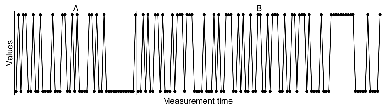
When the dependent variable is dichotomous (e.g., 0 or 1; yes or no), we can estimate a logistic regression. Logistic regression is essentially a special case of binomial regression, applied under the “extreme” condition that there is only one trial per measurement—so that each observation results in either 0% (failure) or 100% (success).

Here is an example dataset with a respective analysis:

plm(example_dichotomous, family = "binomial", var_trials = 1)

Piecewise Regression Analysis

Contrast model: W / level = first, slope = first

Fitted a binomial distribution.
X²(3) = 5.91; p = 0.116; AIC = 205.503

               B LL-CI95% UL-CI95%    SE      t     p    OR  LL-CI95%  UL-CI95%
Intercept -0.174   -1.356    0.972 0.584 -0.298 0.766 0.840     0.258     2.643
Trend     -0.029   -0.075    0.014 0.022 -1.298 0.194 0.971     0.928     1.014
Level B    1.390   -0.114    3.067 0.801  1.734 0.083 4.015     0.892    21.477
Slope B    0.031   -0.014    0.079 0.023  1.333 0.183 1.031     0.986     1.082

Formula: values/1 ~ 1 + mt + phaseB + interB
weights = 1 

10.6.4 Bounded frequencies

In many cases, frequency data are collected without a predetermined upper limit. For example, in a study measuring the frequency of inappropriate classroom behavior, researchers may observe lessons and count the number of disturbances. Although there may be a practical upper limit on the number of possible disturbances, the theoretical limit is infinite.

Another example is a study counting the number of lorries driving on a specific street. Here too, the highest possible number is undefined.

For this type of data, a Poisson distribution is more appropriate. To specify a Poisson model, set the family argument in the plm() function to "poisson".

The following example shows a dataset of injured people due to an accident on an autobahn before and after implementing a speed limit:

Single case data frame for case A24
injuries	year	phase
239	1996	A
263	1997	A
264	1998	A
277	1999	A
283	2000	A
296	2001	A
228	2002	A
136	2003	B
133	2004	B
106	2005	B
123	2006	B
96	2007	B
97	2008	B
103	2009	B
138	2010	B
129	2011	B
136	2012	B
142	2013	B
113	2014	B
177	2015	B
151	2016	B
106	2017	B
71	2018	B
Note. Number of injuries on a German autobahn before and after implementation of a speedlimit (130km/h). Author: Ministerium fuer Infrastruktur und Landesplanung. Land Brandenburg..

Here, a Possion regression is applied:

plm(example_A24, family = "poisson")

Piecewise Regression Analysis

Contrast model: W / level = first, slope = first

Fitted a poisson distribution.
X²(3) = 547.67; p = 0.000; AIC = 261.2856

               B LL-CI95% UL-CI95%    SE       t     p      OR  LL-CI95%
Intercept  5.556    5.472    5.638 0.042 131.693 0.000 258.786   237.936
Trend      0.007   -0.016    0.030 0.012   0.604 0.546   1.007     0.984
Level B   -0.806   -0.938   -0.674 0.067 -11.964 0.000   0.447     0.391
Slope B   -0.006   -0.031    0.019 0.013  -0.472 0.637   0.994     0.969
           UL-CI95%
Intercept   280.900
Trend         1.030
Level B       0.510
Slope B       1.019

Formula: injuries ~ 1 + year + phaseB + interB 

10.7 Model comparison (since version 0.64.0)

The anova function call

anova(object, …)

You can compare the fit of piecewise linear regression (plm) models using the anova() function. This allows for stepwise regression analyses and targeted comparisons (e.g., assessing the combined effect of slope and level changes).

Let’s consider an example where we begin with a null model that includes only an intercept but no additional predictors. We then sequentially add a level effect, followed by a trend effect, and finally a slope effect.

mod0 <- plm(exampleAB$Anja, trend = FALSE, level = FALSE, slope = FALSE)
mod1 <- plm(exampleAB$Anja, trend = FALSE, level = TRUE, slope = FALSE)
mod2 <- plm(exampleAB$Anja, trend = TRUE, level = TRUE, slope = FALSE)
mod3 <- plm(exampleAB$Anja, trend = TRUE, level = TRUE, slope = TRUE)

We start by comparing the null model to the first model:

anova(mod0, mod1)

Analysis of Deviance Table

Model 1: values ~ 1
Model 2: values ~ 1 + phaseB
  Resid. Df Resid. Dev Df Deviance      F    Pr(>F)    
1        19    2410.95                                 
2        18     840.13  1   1570.8 33.655 1.697e-05 ***
---
Signif. codes:  0 '***' 0.001 '**' 0.01 '*' 0.05 '.' 0.1 ' ' 1

The output provides the residuals degrees of freedom (Df), the deviance of the residuals, and \(\Delta Df\) and \(\Delta \text{Deviance}\), which are the difference of the degrees of freedom and the residual deviance of the respective model and the preceding model (here: \(\Delta \text{Df}=19 - 18 = 1\) and \(\Delta \text{Deviance}=2410.95 - 840.13 = 1570.8\)). Deviance is a measure of a model’s goodness of fit and is calculated as \(-2 \times \text{Likelihood}\) . The test compares the difference in degrees of freedom (\(\Delta Df = 1\)) and deviance (\(\Delta \text{Deviance} = 1570.8\)) between the two models.

Since both models assume Gaussian-distributed data, an F-test is performed. The F-value is computed as:

\[ F = \frac{\text{Explained variance}}{\text{Residual variance}} = \frac{\Delta \text{Deviance}}{\text{Residual deviance} / Df} = \frac{1570.8}{\frac{840.13}{18}} = \frac{1570.8}{46.67389} = 33.655 \]

For \(F(1, 18) = 33.655\), the p-value can be obtained with:

pf(33.655,1,18, lower.tail = FALSE)

[1] 1.697306e-05

Alternatively, we can conduct a likelihood-ratio test by setting the argument test = "LRT":

anova(mod0, mod1, test = "LRT")

Analysis of Deviance Table

Model 1: values ~ 1
Model 2: values ~ 1 + phaseB
  Resid. Df Resid. Dev Df Deviance  Pr(>Chi)    
1        19    2410.95                          
2        18     840.13  1   1570.8 6.581e-09 ***
---
Signif. codes:  0 '***' 0.001 '**' 0.01 '*' 0.05 '.' 0.1 ' ' 1

This computes a \(\chi^2\) test for \(\frac{\Delta \text{Deviance}}{\text{Dispersion}} = 33.655\) with \(\Delta Df = 1\), where the p-value is given by:

pchisq(33.655, 1, lower.tail = FALSE)

[1] 6.580551e-09

We can also compare all four models as incrementally nested models in a single step:

anova(mod0, mod1, mod2, mod3)

Analysis of Deviance Table

Model 1: values ~ 1
Model 2: values ~ 1 + phaseB
Model 3: values ~ 1 + mt + phaseB
Model 4: values ~ 1 + mt + phaseB + interB
  Resid. Df Resid. Dev Df Deviance       F    Pr(>F)    
1        19    2410.95                                  
2        18     840.13  1  1570.82 52.1722 2.033e-06 ***
3        17     542.08  1   298.06  9.8994  0.006243 ** 
4        16     481.73  1    60.34  2.0043  0.176029    
---
Signif. codes:  0 '***' 0.001 '**' 0.01 '*' 0.05 '.' 0.1 ' ' 1

Each model is compared to its predecessor. Since all models are nested and derived from the same data, the dispersion parameter for all comparisons is taken from the most complex model, here mod3 (dispersion = 30.11).

In this analysis, we observe that the phase predictor introduces the strongest improvement in model fit, whereas the slope predictor does not significantly enhance the model.

10.8 Dummy models

The model argument is used to code the dummy variables. These dummy variables are used to compute the slope and level effects of the phase variable.
The phase variable is categorical, identifying the phase of each measurement. Typically, categorical variables are implemented by means of dummy variables. In a piecewise regression model two phase effects have to be estimated: a level effect and a slope effect. The level effect is implemented quite straight forward: for each phase beginning with the second phase a new dummy variable is created with values of zero for all measurements except the measurements of the phase in focus where values of one are set.

values	phase	mt	level B
3	A	1	0
6	A	2	0
4	A	3	0
7	A	4	0
5	B	5	1
3	B	6	1
4	B	7	1
6	B	8	1
3	B	9	1

For estimating the slope effect of each phase, another kind of dummy variables have to be created. Like the dummy variables for level effects the values are set to zero for all measurements except the ones of the phase in focus. Here, values start to increase with every measurement until the end of the phase.
Various suggestions have been made regarding the way in which these values increase (see Huitema & Mckean, 2000). The B&L-B model starts with a one at the first session of the phase and increases with every session while the H-M model starts with a zero.

				slope B
values	phase	mt	level B	model B&L-M	model H-M
3	A	1	0	0	0
6	A	2	0	0	0
4	A	3	0	0	0
7	A	4	0	0	0
5	B	5	1	1	0
3	B	6	1	2	1
4	B	7	1	3	2
6	B	8	1	4	3
3	B	9	1	5	4

Applying the H-M model will give you a “pure” level-effect while the B&L-B model will provide an estimation of the level-effect that is actually the level-effect plus on times the slope-effect (as the model assumes that the slope variable is 1 at the first measurement of the B-phase). For most studies, the H-M model is more appropriate.

However, there is another aspect to be aware of. Usually, in single case designs, the measurement times are coded as starting with 1 and increasing in integers (1, 2, 3, …). At the same time, the estimation of the trend effect is based on the measurement time variable. In this case, the estimate of the model intercept (usually interpreted as the value at the beginning of the study) actually represents the estimate of the starting value plus one times the trend effect. Therefore, I have implemented the W model (since scan version 0.54.4). Here the trend effect is estimated for a time variable shifted to start at 0. As a result, the intercept represents the estimated value at the first measurement of the study. The W model treats slope estimation in the same way as the H-M model. That is, the measurement-time for calculating the slope effect is set to 0 for the first session of each phase. Since scan version 0.54.4 the W model is the default.

			mt		slope
values	phase	level	B&L-M and H-M	W	B&L-M	H-M and W
3	A	0	1	0	0	0
6	A	0	2	1	0	0
4	A	0	3	2	0	0
7	A	0	4	3	0	0
5	B	1	5	4	1	0
3	B	1	6	5	2	1
4	B	1	7	6	3	2
6	B	1	8	7	4	3
3	B	1	9	8	5	4

10.9 Designs with more than two phases: Setting the right contrasts

For single case studies with more than two phases, things get a bit more complicated. Applying the models described above to three phases would result in a comparison between each phase and the first phase (usually phase A). That is, the regression weights and significance tests indicate the differences between each phase and the values from phase A. Another common use is to compare the effects of a phase with the previous phase.

As of scan version 0.54.4, plm allows to set a contrast argument. contrast = "first" (the default) will compare all slope and level-effects to the values in the first phase. contrast = "preceding" will compare the slope and level-effects to the preceding phase.

For the preceding contrast, the dummy variable for the level-effect is set to zero for all phases preceding the phase in focus and set to one for all remaining measurements. Similarly, the dummy variable for the slope-effect is set to zero for all phases preceding the phase in focus and starts at zero (or one, depending on the model setting, see Section 10.8) for the first measurement of the target phase and increases until the last measurement of the case.

You can set the contrast differently for the level and slope effects with the arguments constrast_level and contrast_slope. Both can be either "first" or "preceding".

(Note: Prior to scan version 0.54.4, the option model = "JW" was identical to model = "B&L-B", contrast = "preceding").

			contrast first				contrast preceeding
			level		slope		level		slope
values	phase	mt	B	C	B	C	B	C	B	C
3	A	1	0	0	0	0	0	0	0	0
6	A	2	0	0	0	0	0	0	0	0
4	A	3	0	0	0	0	0	0	0	0
7	A	4	0	0	0	0	0	0	0	0
5	B	5	1	0	1	0	1	0	1	0
3	B	6	1	0	2	0	1	0	2	0
4	B	7	1	0	3	0	1	0	3	0
6	B	8	1	0	4	0	1	0	4	0
3	B	9	1	0	5	0	1	0	5	0
7	C	10	0	1	0	1	1	1	6	1
5	C	11	0	1	0	2	1	1	7	2
6	C	12	0	1	0	3	1	1	8	3
4	C	13	0	1	0	4	1	1	9	4
8	C	14	0	1	0	5	1	1	10	5

10.10 Understanding and interpreting contrasts

In this section, we will calculate four plm models with different contrast settings for the same single-case data.

The example scdf is the case ‘Marie’ from the exampleABC scdf (exampleABC$Marie)

Figure 10.3: Example dataset

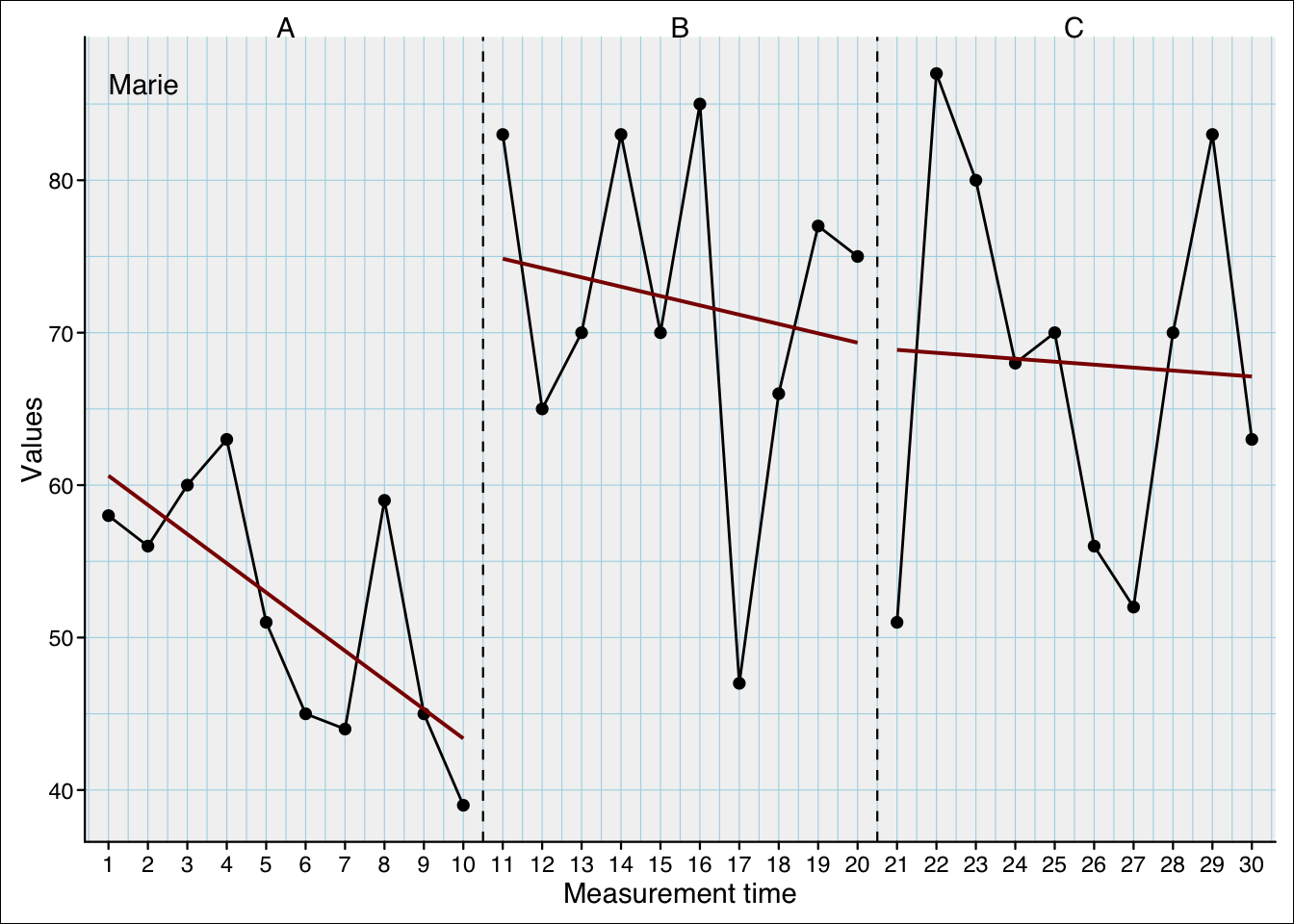
The dark-red lines indicate the intercept and slopes when calculated separately for each phase. They are:

Table 10.1: Intercept, slope, and number of measurements calculated separately for each phase

	intercept	slope	n
phase A	60.618	-1.915	10
phase B	74.855	-0.612	10
phase C	68.873	-0.194	10

Now we estimate a plm model with four contrast settings (see Table 10.2):

Table 10.2: Estimates of a piecewise-linear regression with contrast models “first” and “preceding”.

Contrast level	Contrast slope	intercept	trend	level B	level C	slope B	slope C
first	first	60.618	-1.915	33.388	46.558	1.303	1.721
preceding	preceding	60.618	-1.915	33.388	0.139	1.303	0.418
first	preceding	60.618	-1.915	33.388	33.527	1.303	0.418
preceding	first	60.618	-1.915	33.388	13.170	1.303	1.721

10.10.1 Phase B estimates

All regression models in Table 10.2 have the same estimates for intercept and trend. These are not affected by the contrasts and are identical to those for phase A in Table 10.1. In addition, in Table 10.2, the estimates for levelB and slopeC are identical since all models contrast the same phase (the first and the preceding phase are both phase A). The values here can be calculated from Table 10.1²:

\[ levelB = intercept_{phaseB} - (intercept_{phaseA} + n_{PhaseA} * slope_{phaseA}) \tag{10.1}\]

\[ 33.388 \approx 74.855 - (60.618 + 10*-1.915) \]

\[ slopeB = slope_{phaseB} - slope_{phaseA} \tag{10.2}\]

\[ 1.303 \approx -1.915 - (-0.612) \]

10.10.2 Phase C estimates

The levelC and slopeC estimates of the regression models in Table 10.2 are different for the various contrast models. Depending on the contrast setting, the estimates “answer” a different question. Table 10.3 provides interpretation help.

Table 10.3: Interpretations of the effect estimates in various contrast conditions

Contrast level	Contrast slope	Interpretation of level C effect	Interpretation slope C effect
first	first	What would be the value if phase A had continued until to the start of phase C and what is the difference to the actual value at the first measurement of phase C?	What is the difference between the slopes of phase C and A3?
preceding	preceding	What would be the value if phase B had continued to the start of phase C and what is the difference to the actual value at the first measurement of phase C?	What is the difference between the slopes of phase C and B?
first	preceding	What would be the value if phase A had continued until the start of phase C (assuming a slope effect but no level effect in phase B)? And what is the difference to the actual value at the first measurement of phase C?	What is the difference between the slopes of phase C and B?
preceding	first	What would be the value if phase B had continued until the start of phase C (assuming a level but no slope effect in phase B)? And what is the difference to the actual value at the first measurement of phase C?	What is the difference between the slopes of phase C and A?

All four models are mathematically equivalent, i.e. they produce the same estimates of the dependent variable. Bellow I will show how the estimates from the piecewise regression models relate to the simple regression estimates from Table 10.1. These are \(intercept_{phaseC} = 68.873\) and \(slope_{phaseC} = -0.194\).

Level first and slope first contrasts

Table 10.2 estimates a levelC increase of 46.558 compared to phase A (the intercept) and a slopeC increase of 1.721.

\[ levelC = intercept_{phaseC} - (Intercept_{phaseA} + n_{phaseA+B} * slope_{phaseA}) \tag{10.3}\]

\[46.558 \approx 68.873 - (60.618 + 20*-1.915) \]

\[ slopeC = slope_{phaseC} - slope_{phaseA} \tag{10.4}\]

\[1.721 \approx -0.194 - (-1.915)\]

Level preceding and slope preceding contrasts

Table 10.2 estimates a levelC increase of 0.139 compared to phase B and a slopeC increase of 0.418.

\[ levelC = intercept_{phaseC} - (intercept_{phaseB} + n_{phaseB} * slope_{phaseB}) \tag{10.5}\]

\[0.139 \approx 68.873 - (74.855 + 10*-0.612)\]

\[ slopeC = slope_{phaseC} - slope_{phaseB} \tag{10.6}\]

\[0.418 \approx -0.194 - (-0.612)\]

Level first and slope preceding contrasts

Table 10.2 estimates a levelC increase of 33.388 compared to phase A and a slopeC increase of 0.418.

\[ levelC = intercept_{phaseC} - (intercept_{phaseA} + n_{phaseA} * slope_{phaseA} + n_{phaseB} * slope_{phaseB}) \tag{10.7}\]

\[ 33.527 \approx 68.873 - (60.618 + 10 * -1.915 + 10 * -0.612) \]

\[ slopeC = slope_{phaseC} - slope_{phaseB} \tag{10.8}\]

\[0.418 \approx -0.194 - (-0.612)\]

Level preceding and slope first contrasts

Table 10.2 estimates a levelC increase of 13.170 compared to phase B and a slopeC increase of 1.721.

\[ levelC = intercept_{phaseC} - (intercept_{phaseB} + n_{phaseB} * slope_{phaseA}) \tag{10.9}\]

\[ 13.170\approx 68.873 - (74.855 + 10*-1.915) \]

\[ slopeC = slope_{phaseC} - slope_{phaseA} \tag{10.10}\]

\[ 1.721 \approx -0.194 - (-1.915) \]

Huitema, B. E., & Mckean, J. W. (2000). Design specification issues in time-series intervention models. Educational and Psychological Measurement, 60(1), 38–58. Retrieved from http://epm.sagepub.com/content/60/1/38.short

Wilbert, J., Lüke, T., & Börnert-Ringleb, M. (2022). Statistical power of piecewise regression analyses of single-case experimental studies addressing behavior problems. Frontiers in Education Educational Psychology, 7. https://doi.org/10.3389/feduc.2022.917944

---

1. The session is the ordinal number (1st, 2nd, 3rd, …) of the measurements. While the measurement-time (the value of the measurement-time variable at a specific session/ measurement) is often identical to the session number, this is not necessarily the case. The measurement-time sometimes represents days since the start of the study or other intervals. Therefore, I refer to session or measurement for the ordinal position of the measurement and measurement-time for the value of the time variable at that session number.

2. Differences here and in the following calculations are due to rounding errors.

3. The slope of phase A is the trend effect.