12  Multivariate piecewise regression

Note

Read Chapter 10 before you start with this chapter.

The mplm function call

mplm(data, dvar, mvar, pvar, model = c(“W”, “H-M”, “B&L-B”, “JW”), contrast = c(“first”, “preceding”), contrast_level = c(NA, “first”, “preceding”), contrast_slope = c(NA, “first”, “preceding”), trend = TRUE, level = TRUE, slope = TRUE, formula = NULL, update = NULL, na.action = na.omit, …)

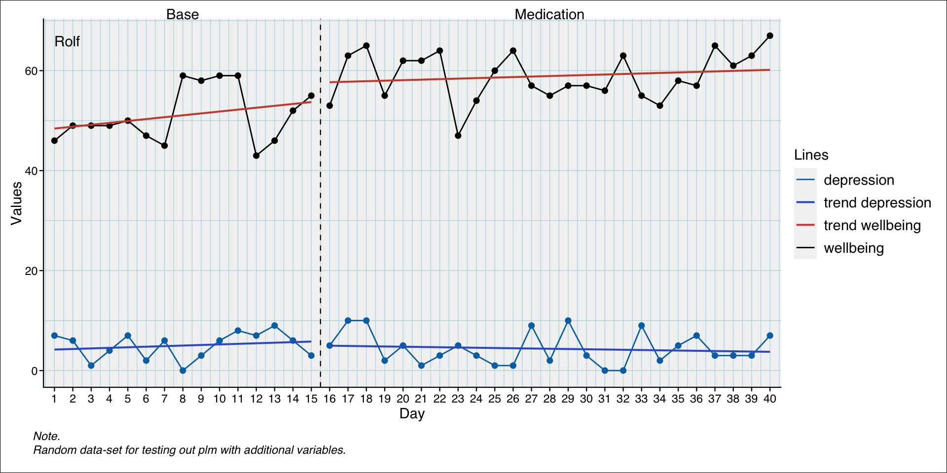
fit <- mplm(exampleAB_add, dvar = c("wellbeing", "depression"))
fit

Multivariate piecewise linear model

Dummy model: W level = first, slope = first

Coefficients: 
                                         wellbeing depression
Intercept                                   48.417      4.200
Trend (day)                                  0.379      0.114
Level phase Medication (phaseMedication)     3.588     -0.945
Slope phase Medication (interMedication)    -0.275     -0.165

Formula: y ~ 1 + day + phaseMedication + interMedication

Type III MANOVA Tests: Pillai test statistic
                                         Df test stat approx F num Df den Df
Intercept                                 1     0.915    188.9      2     35
Trend (day)                               1     0.055      1.0      2     35
Level phase Medication (phaseMedication)  1     0.033      0.6      2     35
Slope phase Medication (interMedication)  1     0.039      0.7      2     35
                                         Pr(>F)    
Intercept                                <2e-16 ***
Trend (day)                                0.38    
Level phase Medication (phaseMedication)   0.56    
Slope phase Medication (interMedication)   0.50    
---
Signif. codes:  0 '***' 0.001 '**' 0.01 '*' 0.05 '.' 0.1 ' ' 1

The following variables were used in this analysis:
'wellbeing/ depression' as dependent variable, 'phase' as phase variable, and 'day' as measurement-time variable.

print(fit, std = TRUE)

Multivariate piecewise linear model

Dummy model: W level = first, slope = first

Coefficients: 
                                         wellbeing depression
Intercept                                   48.417      4.200
Trend (day)                                  0.379      0.114
Level phase Medication (phaseMedication)     3.588     -0.945
Slope phase Medication (interMedication)    -0.275     -0.165

Standardized coefficients: 
                                         wellbeing depression
Intercept                                    0.000      0.000
Trend (day)                                  0.694      0.441
Level phase Medication (phaseMedication)     0.276     -0.153
Slope phase Medication (interMedication)    -0.356     -0.449

Formula: y ~ 1 + day + phaseMedication + interMedication

Type III MANOVA Tests: Pillai test statistic
                                         Df test stat approx F num Df den Df
Intercept                                 1     0.915    188.9      2     35
Trend (day)                               1     0.055      1.0      2     35
Level phase Medication (phaseMedication)  1     0.033      0.6      2     35
Slope phase Medication (interMedication)  1     0.039      0.7      2     35
                                         Pr(>F)    
Intercept                                <2e-16 ***
Trend (day)                                0.38    
Level phase Medication (phaseMedication)   0.56    
Slope phase Medication (interMedication)   0.50    
---
Signif. codes:  0 '***' 0.001 '**' 0.01 '*' 0.05 '.' 0.1 ' ' 1

The following variables were used in this analysis:
'wellbeing/ depression' as dependent variable, 'phase' as phase variable, and 'day' as measurement-time variable.