This chapter describes the multilevel data analyses with a frequentist approach. scan also provides functions for Bayesian analyses that are described in chapter Chapter 13
Read Chapter 10 before you start with this chapter.
Multilevel analyses can take the piecewise-regression approach even further. It allows for
analyzing the effects between phases for multiple single-cases at once
describing variability between subjects regarding these effects, and
introducing variables and factors for explaining the differences.
The basic function for applying a multilevel piecewise regression analysis is hplm (hierarchical piecewise linear model). The hplm function is similar to the plm function, so I recommend that you get familar with plm before applying an hplm.
Here is a simple example:
hplm(exampleAB_50)
Hierarchical Piecewise Linear Regression

Estimation method ML
Contrast model: W / level: first, slope: first
50 Cases

AIC = 8758.802, BIC = 8790.185
ICC = 0.287; L = 339.0; p = 0.000

Fixed effects (values ~ 1 + mt + phaseB + interB)

                            B    SE   df      t p
Intercept              48.398 1.484 1328 32.611 0
Trend (mt)              0.579 0.116 1328  5.006 0
Level phase B (phaseB) 14.038 0.655 1328 21.436 0
Slope phase B (interB)  0.902 0.119 1328  7.588 0

Random effects (~1 | case)

             SD
Intercept 9.970
Residual  5.285
The fixed effects describe the overall effect of the respective predictors on the dependent variable, while the random effects describe the variability of the respective predictor between cases. Here, the fixed effect of the intercept is 48.398 which estimates the mean value across all cases at the first measurement. The standard deviation of this average between cases is 9.97.
In this analysis, we have a basic random intercept model. That is, only the intercept is assumed to vary between cases, whereas the other predictors (Trend, Level, and Slope) are assumed to be identical for all cases.
11.0.1 Explained variance by the variability between cases
The intraclass correlation (ICC) represents the proportion of total variance in the model that is explained by differences between cases.
It is calculated by comparing the model fit (likelihood) of two models using a likelihood ratio test. The first model includes both a fixed and a random intercept as predictors of the measurement, while the second model includes only a fixed intercept without a random intercept.
The model above reports ICC = 0.287; L = 339.0; p = 0.000. This means that approximately 29% of the total variance in the dependent variable is explained by differences between cases, and this variance is statistically significantly greater than 0%.
11.0.2 Variation of single predictors between cases
A multilevel model that includes the variation of specific predictors between cases (e.g., the trend effect) is - in the multilevel regression “world” - called a random slope model.
Here is an example inlcuding random slopes by setting the respective function argument for the trend, slope, and level effects to TRUE:
Hierarchical Piecewise Linear Regression

Estimation method ML
Contrast model: W / level: first, slope: first
50 Cases

AIC = 8693.218, BIC = 8771.677
ICC = 0.287; L = 339.0; p = 0.000

Fixed effects (values ~ 1 + mt + phaseB + interB)

                            B    SE   df      t p
Intercept              48.211 1.398 1328 34.497 0
Trend (mt)              0.621 0.113 1328  5.516 0
Level phase B (phaseB) 13.872 0.894 1328 15.513 0
Slope phase B (interB)  0.864 0.116 1328  7.433 0

Random effects (~1 + mt + phaseB + interB | case)

                          SD
Intercept              9.352
Trend (mt)             0.096
Level phase B (phaseB) 4.537
Slope phase B (interB) 0.126
Residual               4.974

Correlation:
                       Intercept Trend (mt) Level phase B (phaseB)
Trend (mt)                  0.23
Level phase B (phaseB)      0.06      -0.58
Slope phase B (interB)     -0.23      -0.64                  -0.03
The random part of this output now provides estimations of the between case variance of all predictors.
Additionally, we get a correlation matrix of the random slope variables. This depicts the interaction effect of the respective variables at the between case level on the dependent variable. For example, the model above shows a correlation of intercept and trend of r = 0.23. That is, the higher the intercept of a case (the starting value), the stronger the trend effect (here a medium effect size).
Caution
Do not be confused by the terminology: In multilevel regression models, a random slope model refers to the variability of a predictor in a regression model. These predictors contribute to the slope of a linear regression line.
This terminology is used in general within multilevel models, regardless of whether they are applied to single-case studies or not.
In single-case piecewise regressions, the slope effect refers to the difference in the slopes of the regression lines between two phases.
That is, unfortunately, we have a random slope effect of the slope effect!
11.0.3 Testing the random slope variance
It is possible to test the statistical significance of the random slope variances by comparing the overall fit of the model (likelihood) with the fit of the same model without the respective random slope parameter using a likelihood ratio test. To do this, set the argument lr.test = TRUE.
Hierarchical Piecewise Linear Regression

Estimation method ML
Contrast model: W / level: first, slope: first
50 Cases

AIC = 8693.218, BIC = 8771.677
ICC = 0.287; L = 339.0; p = 0.000

Fixed effects (values ~ 1 + mt + phaseB + interB)

                            B    SE   df      t p
Intercept              48.211 1.398 1328 34.497 0
Trend (mt)              0.621 0.113 1328  5.516 0
Level phase B (phaseB) 13.872 0.894 1328 15.513 0
Slope phase B (interB)  0.864 0.116 1328  7.433 0

Random effects (~1 + mt + phaseB + interB | case)

                          SD       L df     p
Intercept              9.352 348.849  4 0.000
Trend (mt)             0.096   0.826  4 0.935
Level phase B (phaseB) 4.537  42.822  4 0.000
Slope phase B (interB) 0.126   0.761  4 0.944
Residual               4.974

Correlation:
                       Intercept Trend (mt) Level phase B (phaseB)
Trend (mt)                  0.23
Level phase B (phaseB)      0.06      -0.58
Slope phase B (interB)     -0.23      -0.64                  -0.03
Here, we can see that the random intercept and the random slope effect for Level phase B are significant. This means that cases have significantly different starting values at the first measurement, and the level intervention effect is also not the same for all cases.
11.0.4 Adding additional L2-variables
TipThe add_l2 function call:
add_l2(scdf, data_l2, cvar = “case”)
In some analyses researchers want to investigate whether attributes of the individuals contribute to the effectiveness of an intervention. For example might an intervention on mathematical abilities be less effective for student with a migration background due to too much language related material within the training. Such analyses can also be conducted with scan. Therefore, we need to define a new data frame including the relevant information of the subjects of the single-case studies we want to analyze. This data frame consists of a variable labeled case which has to correspond to the case names of the scfd and further variables with attributes of the subjects. To build a data frame we can use the R function data.frame.
L2 <-data.frame(case =c("Antonia","Theresa", "Charlotte", "Luis", "Bennett", "Marie"), age =c(16, 13, 13, 10, 5, 14), sex =c("f","f","f","m","m","f"))L2
       case age sex
1   Antonia  16   f
2   Theresa  13   f
3 Charlotte  13   f
4      Luis  10   m
5   Bennett   5   m
6     Marie  14   f
Multilevel analyses require a high number of Level 2 units. The exact number depends on the complexity of the analyses, the size of the effects, the number of level 1 units, and the variability of the residuals. But surely we need at least about 30 level 2 units. In a single-case design that is, we need at least 30 single-cases (subjects) within the study. After setting the level 2 data frame we can merge it to the scdf with the add_l2() function (alternatively, we can use the data.l2 argument of the hplm function). Then we have to specify the regression function using the update.fixed argument. The level 2 variables can be added just like any other additional variable. For example, we have added a level 2 data-set with the two variables sex and age. update could be construed of the level 1 piecewise regression model .~. plus the additional level 2 variables of interest + sex + age. The complete argument is update.fixed = .~. + sex + age. This analyses will estimate a main effect of sex and age on the overall performance. In case we want to analyze an interaction between the intervention effects and for example the sex of the subject we have to add an additional interaction term (a cross-level interaction). An interaction is defined with a colon. So sex:phase indicates an interaction of sex and the level effect in the single case study. The complete formula now is update.fixed = .~. + sex + age + sex:phase.
scan includes an example single-case study with 50 subjects example50 and an additional level 2 data-set example50.l2. Here are the first 10 cases of example50.l2.
case
sex
age
Roman
m
12
Brennen
m
10
Ismael
m
13
Donald
m
11
Ricardo
m
13
Izayah
m
11
Ignacio
m
12
Xavier
m
12
Arian
m
10
Paul
m
10
Analyzing the data with hplm could look like this:
exampleAB_50 |>add_l2(exampleAB_50.l2) |>hplm(update.fixed = .~. + sex + age)
Hierarchical Piecewise Linear Regression

Estimation method ML
Contrast model: W / level: first, slope: first
50 Cases

AIC = 8757.458, BIC = 8799.303
ICC = 0.287; L = 339.0; p = 0.000

Fixed effects (values ~ mt + phaseB + interB + sex + age)

                            B     SE   df      t     p
Intercept              44.878 11.926 1328  3.763 0.000
Trend (mt)              0.581  0.116 1328  5.026 0.000
Level phase B (phaseB) 14.023  0.655 1328 21.405 0.000
Slope phase B (interB)  0.900  0.119 1328  7.569 0.000
sexm                   -6.440  2.727   47 -2.362 0.022
age                     0.603  1.073   47  0.562 0.577

Random effects (~1 | case)

             SD
Intercept 9.446
Residual  5.284
sex is a factor with the levels f and m. So sexm is the effect of being male on the overall performance. age does not seem to have any effect. So we drop age out of the equation and add an interaction of sex and phase to see whether the sex effect is due to a weaker impact of the intervention on males.
exampleAB_50 |>add_l2(exampleAB_50.l2) |>hplm(update.fixed = .~. + sex + sex:phaseB)
Hierarchical Piecewise Linear Regression

Estimation method ML
Contrast model: W / level: first, slope: first
50 Cases

AIC = 8604.949, BIC = 8646.794
ICC = 0.287; L = 339.0; p = 0.000

Fixed effects (values ~ mt + phaseB + interB + sex + phaseB:sex)

                                 B    SE   df       t    p
Intercept                   48.573 1.968 1327  24.676 0.00
Trend (mt)                   0.609 0.109 1327   5.573 0.00
Level phase B (phaseB)      17.726 0.684 1327  25.922 0.00
Slope phase B (interB)       0.884 0.112 1327   7.868 0.00
sexm                        -0.593 2.741   48  -0.216 0.83
Level phase B (phaseB):sexm -7.732 0.609 1327 -12.699 0.00

Random effects (~1 | case)

             SD
Intercept 9.494
Residual  4.989
Now the interaction phase:sexm is significant and the main effect is no longer relevant. It looks like the intervention effect is \(7.7\) points lower for male subjects. While the level-effect is \(17.7\) points for female subjects it is \(17.7\) - \(7.7\) = \(10\) for males.
11.0.5 Estimations for each case
For a multilevel model, you can estimate the values for each parameter for each case based on the random intercept and slope values.
Use the casewise argument to access these estimations.
res <-hplm(exampleAB_50[1:10],random.slopes =TRUE)# retrieve the case estimations for further calculationscs <-coef(res, casewise =TRUE)# or print themprint(res, casewise =TRUE)
Hierarchical Piecewise Linear Regression

Estimation method ML
Contrast model: W / level: first, slope: first
10 Cases

AIC = 1799.887, BIC = 1854.674
ICC = 0.327; L = 84.3; p = 0.000

Fixed effects (values ~ 1 + mt + phaseB + interB)

                            B    SE  df      t     p
Intercept              43.775 2.687 272 16.291 0.000
Trend (mt)              0.994 0.299 272  3.330 0.001
Level phase B (phaseB)  8.675 1.745 272  4.971 0.000
Slope phase B (interB)  0.527 0.296 272  1.779 0.076

Random effects (~1 + mt + phaseB + interB | case)

                          SD
Intercept              7.867
Trend (mt)             0.488
Level phase B (phaseB) 3.309
Slope phase B (interB) 0.440
Residual               4.930

Correlation:
                       Intercept Trend (mt) Level phase B (phaseB)
Trend (mt)                  0.86
Level phase B (phaseB)      -0.6      -0.88
Slope phase B (interB)      -0.9      -0.97                   0.75

Casewise estimation of effects

    Case Intercept Trend (mt) Level phase B (phaseB) Slope phase B (interB)
   Roman  43.00890  0.8466415              10.112584             0.61645793
 Brennen  47.43929  1.1041397               9.194792             0.35512806
  Ismael  53.40011  1.7200025               3.193577            -0.01337901
  Donald  56.00259  1.6045806               6.361723            -0.08687239
 Ricardo  43.13287  0.9900639               8.374106             0.54179253
  Izayah  41.47913  0.9871108               8.000154             0.56548397
 Ignacio  47.69657  1.1943236               7.839439             0.32568942
  Xavier  40.65876  0.8529937               9.300791             0.65995521
   Arian  26.77803  0.1614968              11.741146             1.36295987
    Paul  38.15377  0.4785178              12.631557             0.94227384
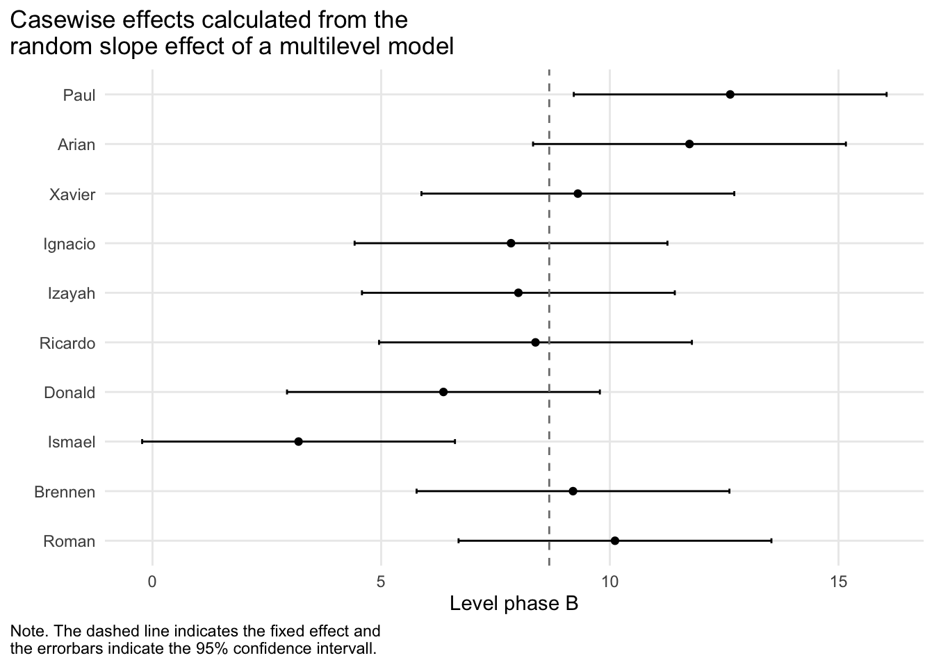
If you have the scplot package installed (version 0.4.1 or higher), you can create a forestplot for each parameter of the model with the scplot() function. Set the argument “effect” to choose the effect by number or a string (“intercept”, “trend”, “slope”, “level”). The ci argument sets the size of the confidence interval (default is 0.95) and the mark argument sets the value for a reference line (default is the mean effect).
library(scplot)scplot(res, effect ="level")
ℹ Possible effects are:
  2: 'Intercept'
  3: 'Trend (mt)'
  4: 'Level phase B (phaseB)'
  5: 'Slope ... [truncated]
`height` was translated to `width`.