library(scan)
library(scplot)
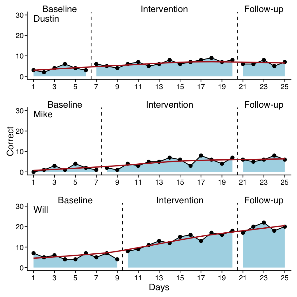
case1 <- scdf(
c(A = 3, 2, 4, 6, 4, 3,
B = 6, 5, 4, 6, 7, 5, 6, 8, 6, 7, 8, 9, 7, 8,
C = 6, 6, 8, 5, 7),
name = "Dustin"
)
case2 <- scdf(
c(A = 0, 1, 3, 1, 4, 2, 1,
B = 2, 1, 4, 3, 5, 5, 7, 6, 3, 8, 6, 4, 7,
C = 6, 5, 6, 8, 6),
name = "Mike"
)
case3 <- scdf(
c(A = 7, 5, 6, 4, 4, 7, 5, 7, 4,
B = 8, 9, 11, 13, 12, 15, 16, 13, 17, 16, 18,
C = 17, 20, 22, 18, 20),
name = "Will"
)
strange_study <- c(case1, case2, case3)1 Introduction
Note
You will need a basic degree of familiarity with the R language. Appendix A gives a brief introduction.
Single case research has become an important and widely accepted method for gaining insight into educational processes. In particular, the field of special education has embraced single case research as an appropriate method for evaluating the effectiveness of an intervention or the developmental processes underlying problems in the acquisition of academic skills. Single case studies are also popular with teachers and educators who are interested in evaluating the learning progress of their students. Despite their usefulness, standards for conducting single-case studies, analysing the data, and presenting the results are less well developed than for group-based research designs. Furthermore, while there is a wealth of software available to help analyse data, most of it is designed to analyse group-based datasets. Visualising single case data sets often means fiddling with spreadsheets, and analysis becomes a cumbersome endeavour. This book fills that gap. It has been written around a specialised software tool for managing, visualising and analysing single case data. This tool is an extension package for the R software (R Core Team, 2026) called scan, an acronym for single case analysis.
I am now going to make up some data for this fictitious KUNO study, because it would be too difficult to carry out a real study and actually develop a real intervention method.↩︎