### Three ways to code the same scdf
scdf(values = c(2,2,4,5,8,7,6,9,8,7), phase_starts = c(A = 1, B = 5))
scdf(values = c(2,2,4,5,8,7,6,9,8,7), phase_design = c(A = 4, B = 6))
scdf(values = c(A = 2,2,4,5, B = 8,7,6,9,8,7))3 Create, display, and store single-case data
3.1 A single-case data frame
Scan provides its own data-class for encoding single-case data: the single-case data frame (short scdf). An scdf is an object that contains one or multiple single-case data sets and is optimized for managing and displaying these data. Think of an scdf as a file including a separate datasheet for each single case. Each datasheet is made up of at least three variables: The measured values, the phase identifier for each measured value, and the measurement time (mt) of each measure. Optionally, scdfs could include further variables for each single-case (e.g., control variables), and also a name for each case.
Note
Technically, an scdf object is a list containing data frames. It is of the class c("scdf","list"). Additionally, an scdf entails an attribute scdf with a list with further attributes. var.values, var.phase, and var.mt contain the names of the values, phase, and the measurement time variable. By default, these names are set to values, phase, and mt.
Several functions are available for creating, transforming, merging, and importing/exporting scdfs.
3.2 Create single-case data frames
TipThe scdf function call:
scdf(
…,
B_start = NULL,
phase_starts = NULL,
phase_design = NULL,
name = NULL,
dvar = “values”,
pvar = “phase”,
mvar = “mt”
)
The scdf() function is the basic tool for creating a single-case data frame. Basically, you have to provide the measurement values and the phase structure and an scdf object is build. There are three different ways of defining the phase structure. First, defining the beginning of each phase with the phase_starts argument, second, defining a design with the phase_design argument and third, setting parameters in a named vector of the dependent variable.
The phase_starts argument is a named vector with the starts of each phase. The number assigned to phase_starts indicate the measurement-time as defined in the mt argument. That is, assume a vector for the measurement times mt = c(1,3,7,10,15,17,18,20) and phase_starts = c(A = 1, B = 15) then the first measurement of the B-phase will start with the fifth measurement at which mt = 15.
The phase_design argument is a named vector with the name and length of each phase. Here, the values indicate the numbers of measurements (including explicit missing values, the mt argument is not taken into account).
When the vector of the dependent variable includes named values, a phase_design structure is created automatically. Each named value sets the beginning of a new phase. For example c(A = 3,2,4, B = 5,4,3, C = 6,7,6,5) will create an ABC-phase design with 3, 3, and 4 values per phase.
The phase names can be set arbitrary, although I recommend to use capital letters (A, B, C, …) for each phase followed by, when indicated, a number if the phases repeat (A1, B1, A2, B2, …). Although it is possible to give the same name to more than one phase (A, B, A, B) this might lead to some confusion and errors when coding analyzes with scan.
Note
A deprecated argument is B_start which is only applicable when the single-case consists of a single A-phase followed by a B-phase. It is a remnant from the time when scan could only handle one-case designs with two phases. The number assigned to B_start indicates the measurement-time as defined in the mt argument.
If no measurement times are specified, they are automatically created as a series 1, 2, 3, …, N, where N is the number of measurements. in some circumstances it might be useful to define individual measurement times for each measurement. For example, if you want to include the days since the beginning of the study as time intervals between measurements are widely varying you might get more valid results this way when analyzing the data in a regression approach.
# example of a more complex design
scdf(
  values = c(2,2,4,5, 8,7,6,9,8,7, 12,11,13),
  mt = c(1,2,3,6, 8,9,11,12,16,18, 27,28,29),
  phase_design = c(A = 4, B = 6, C = 3)
)
#A single-case data frame with one case
[case #1]: values mt phase
2 1 A
2 2 A
4 3 A
5 6 A
8 8 B
7 9 B
6 11 B
9 12 B
8 16 B
7 18 B
12 27 C
11 28 C
13 29 CMissing values could be coded using NA (not available).
scdf(values = c(A = 2,2,NA,5, B = 8,7,6,9,NA,7))More variables are implemented by adding new variable names with a vector containing the values. Please be aware that a new variable must never have the same name as one of the arguments of the function (i.e. phase_starts, phase_design, name, dvar, pvar, mvar).
scdf(
  values = c(A = 2,2,3,5, B = 8,7,6,9,7,7),
  teacher = c(0,0,1,1,0,1,1,1,0,1),
  hour = c(2,3,4,3,3,1,6,5,2,2)
)
#A single-case data frame with one case
[case #1]: values teacher hour mt phase
2 0 2 1 A
2 0 3 2 A
3 1 4 3 A
5 1 3 4 A
8 0 3 5 B
7 1 1 6 B
6 1 6 7 B
9 1 5 8 B
7 0 2 9 B
7 1 2 10 BTable 3.1 shows a complete list of arguments that could be passed to the function.
| Argument | What it does ... |
|---|---|
| values | The default vector with values for the dependent variable. It can be changed with the dvar argument. |
| phase | Usually, this variable is not defined manually and will be created by the function. It is the default vector with values for the phase variable. It can be changed with the pvar argument. |
| mt | The default vector with values for the measurement-time variable. It can be changed with the mvar argument. |
| phase_design | A named vector defining the length and label of each phase. |
| phase_starts | A named vector defining the startpoint of each phase with respect to the measurement-time. |
| (deprecated) B_start | The first measurement of phase B (simple coding if design is strictly AB). |
| name | A name for the case. |
| dvar | The name of the dependent variable. By default this is 'values'. |
| pvar | The name of the variable containing the phase information. By default this is 'phase'. |
| mvar | The name of the variable with the measurement-time. The default is 'mt'. |
| ... | Any number of variables with a vector asigned to them. |
If you want to create a dataset comprising several single cases, the easiest way is to first create an scdf for each case and then merge them into a new scdf using the c command:
case1 <- scdf(
  values = c(A = 5, 7, 10, 5, 12, B = 7, 10, 18, 15, 14, 19),
  name = "Charlotte"
)
case2 <- scdf(
  values = c(A = 3, 4, 3, 5, B = 7, 4, 7, 9, 8, 10, 12),
  name = "Theresa"
)
case3 <- scdf(
  values = c(A = 9, 8, 8, 7, 5, 7, B = 6, 14, 15, 12, 16),
  name = "Antonia"
)
mbd <- c(case1, case2, case3)
If you want to use other than the default variable names (“values”, “phase” and “mt”), you can define them with the arguments dvar (for the dependent variable), pvar (the variable specifying the phase) and mvar (the measurement time variable).
# Example: Using a different name for the dependent variable
case <- scdf(
  score = c(A = 5, 7, 10, 5, 12, B = 7, 10, 18, 15, 14, 19),
  dvar = "score"
)

# Example: Using new names for the dependent and the phase variables
case <- scdf(
  score = c(A = 3, 4, 3, 5, B = 7, 4, 7, 9, 8, 10, 12),
  dvar = "score", pvar = "section"
)

# Example: Using new names for dependent, phase, and measurement-time variables
case <- scdf(
  score = c(A = 9, 8, 8, 7, 5, 7, B = 6, 14, 15, 12, 16),
  name = "Antonia", dvar = "score", pvar = "section", mvar = "day"
)

summary(case)
#A single-case data frame with one case
Measurements Design
Antonia 11 A-B
Variable names:
score <dependent variable>
section <phase variable>
day <measurement-time variable>3.3 Save and read single-case data frames
Normally, it is not necessary to save an scdf in a separate file on your computer. In most cases, you can keep the coding of the scdf as described above and run it again each time you work with your data. However, for large files, it is sometimes more convenient to save the data separately in a file for later use.
The easiest way is to use the R base functions saveRDS and readRDS for this purpose. saveRDS takes at least two arguments: The first is the object you want to save, and the second is a filename for the resulting file. If you have an scdf named study1, you can use saveRDS(study1, "study1.rds") to save the scdf to your drive. You can read this file with study1 <- readRDS("study1.rds"). With getwd() you get the path to the current active folder you are saving and reading data from.
3.4 Import and export single-case data frames
3.4.1 Import data
TipThe read_scdf function call:
read_scdf(
file,
cvar = “case”,
pvar = “phase”,
dvar = “values”,
mvar = “mt”,
sort_cases = FALSE,
phase_names = NULL,
type = NA,
na = c(““,”NA”),
…
)
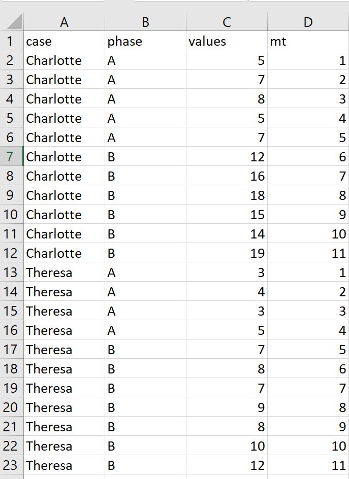
When you are working with other programs besides R you need to export and import the scdf into a common file format. read_scdf imports a comma-separated-variable (csv) file and converts it into an scdf object. By default, the csv-file has to contain the columns case, phase, and values. Optionally, a further column named mt could be provided. The csv file should be build up like this:
In case your variables names differ from the standard (i.e. “case”, “values”, “phase”, and “mt” ), you could set additional arguments to fit your file. read_scdf("example.csv", cvar = "name", dvar = "wellbeing", pvar = "intervention", mvar = "time") for example will set the variables attributes of the resulting scdf. Cases will be split by the variable "name", "wellbeing" is set as the dependent variable (default is values), phase information are in the variable "intervention", and measurement times in the variable "time". You could also reassign the phase names within the phase variable by setting the argument phase_names. Assume for example your file contains the values 0 and 1 to identify the two phases I recommend to set them to “A” and “B” with read_scdf("example.csv", phase_names = c("A", "B")).
For some reasons, computer systems with a German (and some other) language setups export csv-files by default with a comma as a decimal point and a semicolon as a separator between values. In these cases you have to set two extra arguments to import the data:
read_scdf("example.csv", dec = ",", sep = ";")
3.4.2 Other data formats
read_scdf also allows for directly importing Microsoft Excel .xlsx or .xls files. You need to have the library readxl installed in your R setup for this to work. Excel files will be automatically detected by the filename extension xlsor xlsx or by explicitly setting the type argument (e.g. type = "xlsx").
dat <- read_scdf(
  "example2.xlsx", cvar = "name", pvar = "intervention",
  dvar = "wellbeing", mvar = "time", phase_names = c("A","B")
)
Imported 20 casessummary(dat)#A single-case data frame with 20 cases
Measurements Design
Charles 20 A-B
Kolten 20 A-B
Annika 20 A-B
Kaysen 20 A-B
Urijah 20 A-B
Leila 20 A-B
Leia 20 A-B
Aleigha 20 A-B
Greta 20 A-B
Alijah 20 A-B
... [skipped 10 cases]
Variable names:
wellbeing <dependent variable>
intervention <phase variable>
time <measurement-time variable>
age
gender
gymBasically, you can import data from any file format with the help of additional R packages and the as_scdf() function. Here are two examples:
# Open document example. You need to have the readODS package installed.
df <- readODS::read_ods("filename.ods")
scdf <- as_scdf(df)

# SPSS example. You need to have the haven package installed.
df <- haven::read_sav("filename.sav")
scdf <- as_scdf(df)
3.4.3 Export data
TipThe write_scdf function call:
write_scdf(data, filename = NULL, sep = “,”, dec = “.”, …)
write_scdf() exports an scdf object as a comma-separated-variables file (csv) which can be imported into any other software for data analyses (MS OFFICE, Libre Office etc.). The scdf object is converted into a single data frame with a case variable identifying the rows for each subject. The first argument of the command identifies the scdf to be exported and the second argument (file) the name of the resulting csv-file. If no file argument is provided, a dialog box is opened to choose a file interactively. By default, write_scdf exports into a standard csv-format with a dot as the decimal point and a comma for separating variables. If your system expects a comma instead of a point for decimal numbers you may use the dec and the sep arguments. For example, write_scdf(example, file = "example.csv", dec = ",", sep = ";") exports a csv variation usually used for example in Germany.
3.4.4 Other data formats
The R system has many add on packages that allow to write data to almost any file format available. If you like to export an scdf in those formats, you firstly need to convert the scdf into a standard R data-frame with the as.data.frame() function. Now you can export the resulting data-frame applying the respective function from another package.
df <- as.data.frame(exampleABC)

# Open document example. You need to have the readODS package installed.
readODS::write_ods(df, "filename.ods")

# Excel example. You need to have the openxlsx package installed.
openxlsx::write.xlsx(df, "filename.xlsx")

# SPSS example. You need to have the haven package installed.
haven::write_sav(df, "filename.sav")
3.5 Convert an scdf object back to scan syntax
TipThe convert function call:
convert(scdf, file = ““, study_name =”study”, case_name = “case”, inline = FALSE, indent = 2, silent = FALSE)
You can also reconvert an scdf object back to “raw” scan syntax. This is a convenient way when you imported data from an Excel or csv file and want to keep everything clean and transparent within your R syntax files.
Here is an example:
convert(exampleABC)case1 <- scdf(
values = c(
58, 56, 60, 63, 51, 45, 44, 59, 45, 39, 83, 65, 70, 83, 70, 85, 47, 66,
77, 75, 51, 87, 80, 68, 70, 56, 52, 70, 83, 63
),
phase_design = c(A = 10, B = 10, C = 10),
name = "Marie"
)
case2 <- scdf(
values = c(
47, 41, 47, 52, 54, 65, 55, 37, 51, 60, 60, 65, 55, 46, 49, 54, 77, 73,
97, 64, 84, 71, 66, 74, 78, 68, 52, 76, 63, 54
),
phase_design = c(A = 15, B = 8, C = 7),
name = "Rosalind"
)
case3 <- scdf(
values = c(
50, 45, 63, 53, 66, 57, 35, 45, 74, 63, 47, 45, 47, 36, 51, 55, 35, 66,
59, 55, 73, 60, 85, 62, 79, 69, 87, 76, 90, 48
),
phase_design = c(A = 20, B = 7, C = 3),
name = "Lise"
)
study <- c(
case1, case2, case3
) Set inline = TRUE if you prefer the phase definition in a named vector:
convert(exampleABC$Marie, inline = TRUE)study1 <- scdf(
values = c(
A = 58, 56, 60, 63, 51, 45, 44, 59, 45, 39,
B = 83, 65, 70, 83, 70, 85, 47, 66, 77, 75,
C = 51, 87, 80, 68, 70, 56, 52, 70, 83, 63
),
name = "Marie"
)
Now you can copy and past the output into your R file or you set the file argument to save the output into an R file convert(exampleABC, file = "scdf.R").
3.6 Display single-case data frames
TipThe print scdf function call:
print(
x,
cases = getOption(“scan.print.cases”),
rows = getOption(“scan.print.rows”),
cols = getOption(“scan.print.cols”),
long = getOption(“scan.print.long”),
digits = getOption(“scan.print.digits”),
…
)
scdf are displayed by just typing the name of the object.
#Beretvas2008 is an example scdf included in scan
Beretvas2008
#A single-case data frame with one case
[case #1]: values mt phase
0.7 1 A
1.6 2 A
1.4 3 A
1.6 4 A
1.9 5 A
1.2 6 A
1.3 7 A
1.6 8 A
10 9 B
10.8 10 B
11.9 11 B
11 12 B
13 13 B
12.7 14 B
14 15 BThe print command allows you to specify the output. Some possible arguments are cases (the number of cases to display; three by default), rows (the maximum number of rows to display; fifteen by default), and digits (the number of digits). cases = 'all' and rows = 'all' prints all cases and rows.
# Huber2014 is an example scdf included in scan
print(Huber2014, cases = 2, rows = 10)
#A single-case data frame with four cases
Adam: compliance mt phase | Berta: compliance mt phase |
25 1 A | 25 1 A |
20.8 2 A | 20.8 2 A |
39.6 3 A | 39.6 3 A |
75 4 A | 75 4 A |
45 5 A | 45 5 A |
39.6 6 A | 14.6 6 A |
54.2 7 A | 45.8 7 A |
50 8 A | 33.3 8 A |
28.1 9 A | 31.3 9 A |
40 10 A | 32.5 10 A |
# ... up to 66 more rows
# two more casesThe argument long = TRUE prints each case one after the other instead of side by side (e.g., print(exampleAB, long = TRUE)).
3.6.1 Summary
TipThe summary scdf function call:
summary(object, all_cases = FALSE, …)
A short description of the scdf is provided by the summary command. The results are pretty much self explaining:
summary() gives a very concise overview of an scdf
summary(Huber2014)#A single-case data frame with four cases
Measurements Design
Adam 37 A-B
Berta 29 A-B
Christian 76 A-B
David 76 A-B
Variable names:
compliance <dependent variable>
phase <phase variable>
mt <measurement-time variable>
Note: Behavioral data (compliance in percent).
Author of data: Christian Huber