6 Missing values and outliers

6.1 Missing values

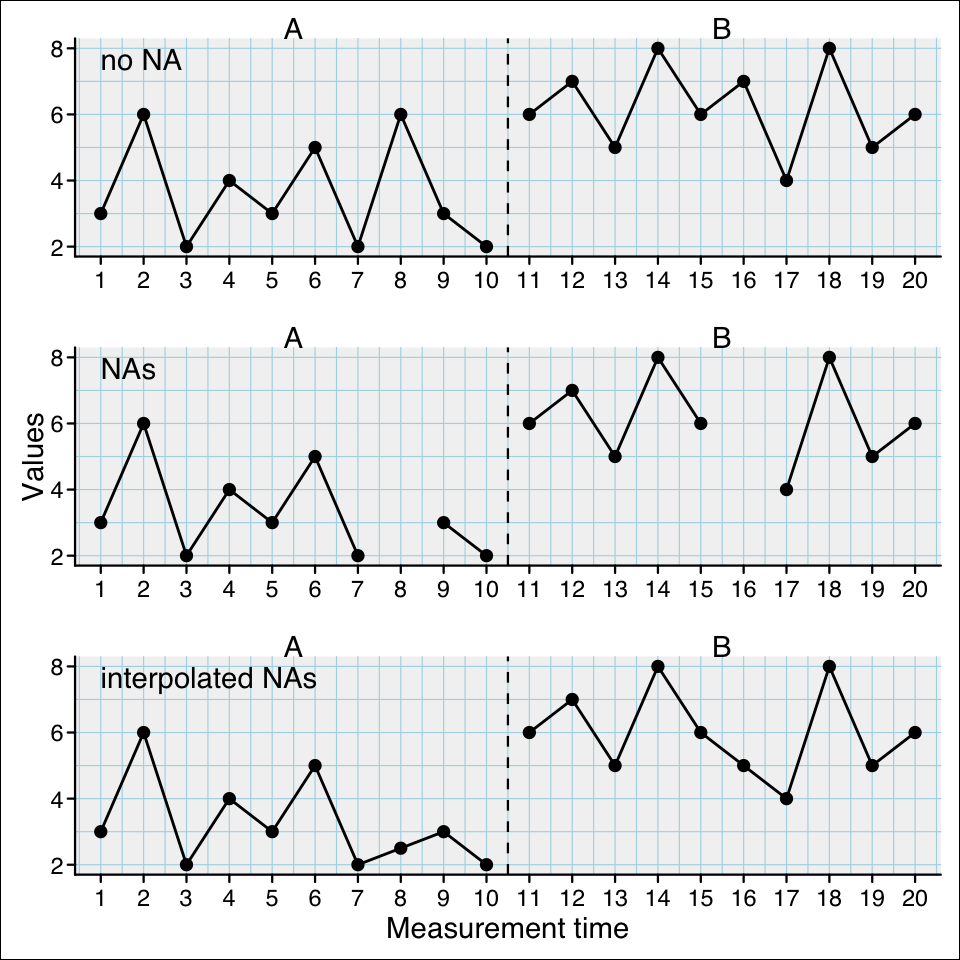
There are two kinds of missing values in single-case data series. First, missings that were explicitly recorded as NA and assigned to a phase and measurement-time as in the following example:

scdf(c(5, 3, 4, 6, 8, 7, 9, 7, NA, 6), phase_design = c(A = 4, B = 6))

The second type of missing occurs when there are gaps between measurement-times that are not explicitly coded as in the following example:

scdf(c(5, 3, 4, 6, 8, 7, 9, 7, 6), phase_design = c(A = 4, B = 5), 
     mt = c(1, 2, 3, 4, 5, 6, 7, 8, 10))

In both cases, missing values pose a threat to the internal validity of overlap indices. Randomization tests are more robust against the first type of missing values but are affected by the second type. Regression approaches are less impacted by both types as they take the interval between measurement-times into account.

case1 <- scdf(c(3,6,2,4,3,5,2,6,3,2, 6,7,5,8,6,7,4,8,5,6), 
              phase_design = c(A = 10, B = 10), name = "no NA")
case2 <- scdf(c(3,6,2,4,3,5,2,NA,3,2, 6,7,5,8,6,NA,4,8,5,6), 
              phase_design = c(A = 10, B = 10), name = "NAs")
case3 <- fill_missing(case2)
names(case3) <- "interpolated NAs"
ex <- c(case1, case2, case3)
scplot(ex)

Warning: Removed 2 rows containing missing values (`geom_point()`).

overlap(ex)

Overlap Indices

Comparing phase 1 against phase 2 

             no NA  NAs interpolated NAs
Design         A-B  A-B              A-B
PND             40   33               30
PEM            100  100              100
PET            100  100              100
NAP             88   91               92
NAP rescaled    77   83               83
PAND            80   89               90
IRD           0.60 0.67             0.70
Tau_U(A)      0.53 0.61             0.61
Tau_U(BA)     0.45 0.51             0.50
Base_Tau      0.59 0.64             0.64
Diff_mean     2.60 2.78             2.75
Diff_trend    0.02 0.11             0.12
SMD           1.65 1.96             2.02
Hedges_g      1.71 1.90             1.96

6.2 Outlieranalysis

The outlier function call

outlier(data, dvar, pvar, mvar, method = c(“MAD”, “Cook”, “SD”, “CI”), criteria = 3.5)

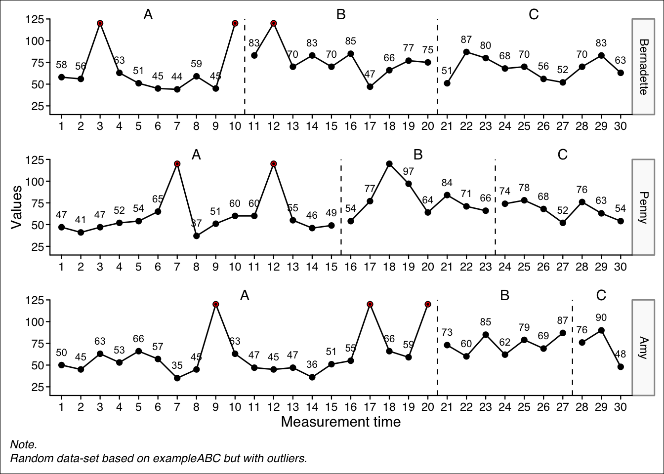
scan provides several methods for analyzing outliers. All of them are implemented in the outliers function. Available methods are the standard deviation, mean average deviation, confidence intervals, and Cook’s distance. The criteria argument takes a vector with two information, the first defines the analyzing method (“SD”, “MAD”, CI”, “Cook”) and the second the criteria. For “SD” the criteria is the number of standard deviations (sd) from the mean of each phase for which a value is not considered to be an outlier. For example, criteria = c("SD",2) would identify every value exceeding two sd above or below the mean as an outlier whereas sd and mean refer to phase of a value. As this might be misleading particularly for small samples Iglewicz and Hoaglin Iglewicz & Hoaglin (1993) recommend the use the much more robust median average deviation (MAD) instead. The MAD is is constructed similar to the sd but uses the median instead of the mean. Multiplying the MAD by 1.4826 approximates the sd in a normal distributed sample. This corrected MAD is applied in the outlier function. A deviation of 3.5 times the corrected MAD from the median is suggested to be an outlier. To use this criterion set criteria = c("MAD", 3.5). criteria = c("CI", 0.95) takes exceeding the 95% confidence interval as the criteria for outliers. The Cook’s distance method for calculation outliers can be applied with a strict AB-phase design. in that case, the Cook’s distance analyses are based on a piecewise-regression model. Most commonly, Cook’s distance exceeding 4/n is used as a criteria. This could be implemented setting criteria = c("Cook","4/n").

outlier(exampleABC_outlier, criteria = c("MAD", 3.5))

Outlier Analysis for Single-Case Data

Case Bernadette : Dropped 3 
Case Penny : Dropped 2 
Case Amy : Dropped 3

# Visualizing outliers with the plot function
res <- outlier(exampleABC_outlier, criteria = c("MAD", 3.5))

scplot(exampleABC_outlier) %>%
  add_labels(nudge_y = 15, text = list(size = 0.7)) %>%
  add_marks(positions = res) %>%
  add_theme("basic") %>%
  set_casenames(position = "strip") %>%
  set_yaxis(limits = c(20, 120))

Warning in add_theme(., "basic"): Deprecated. Please use `set_theme()`

Warning: Removed 9 rows containing missing values (`geom_text()`).